AWS Glue Elastic Views! An almost no code ETL and Aggregation Framework

Introduction

ETL is a fundamental step of a Machine Learning process as it is the stepping stone on which all the dataset for the model definition is based. Because of that, data scientists and MLOps experts carefully plan jobs and pipelines to manage the extraction of data from databases, often of different natures, clean and normalize data, and finally generate a data lake to make further enhancement on data during the investigation process.

Usually, this process involves different steps, coordinating their resolution, accessing different databases with different technologies, preparing many scripts, knowing different languages to query the relevant data, and so on.

Taking care of all these steps is a daring task and requires a lot of expertise, and of course, is time-consuming, undercutting the efficiency of the entire project at hand.

In the last couple of years AWS has been aggressively developing tools and services to help in Machine Learning and ETL tasks and at the last re:Invent introduced another important component for ETL-ML preparation: AWS Elastic Views. 

AWS Elastic Views allows a user to request data from different data sources being completely agnostic on their nature, to query for data in a SQL-compatible language, and to send all the queried data to a target, typically S3 or another data store in order to aggregate the heterogenous data in a data lake.

Some of the main advantages are: 

• being able to query with PartiQL language, databases or datastream of different nature, becoming a defacto aggregator without the need to write custom complex ETL jobs.
• Using powerful commands like JOIN to add aggregation capabilities to data sources that usually don’t have.

The purpose of this article is to guide the reader in exploring some of the key factors that make this service something to consider while drafting your Machine Learning projects.

We’ll dive deep into what AWS Elastic Views is capable of, considering that it is still in the beta private preview phase, so you’ll have to ask AWS access for the preview.

Let’s go! 

How it works

Let’s start our journey by understanding what is AWS Glue Elastic Views, and how it works. At first, let’s take a look at this scheme by AWS:

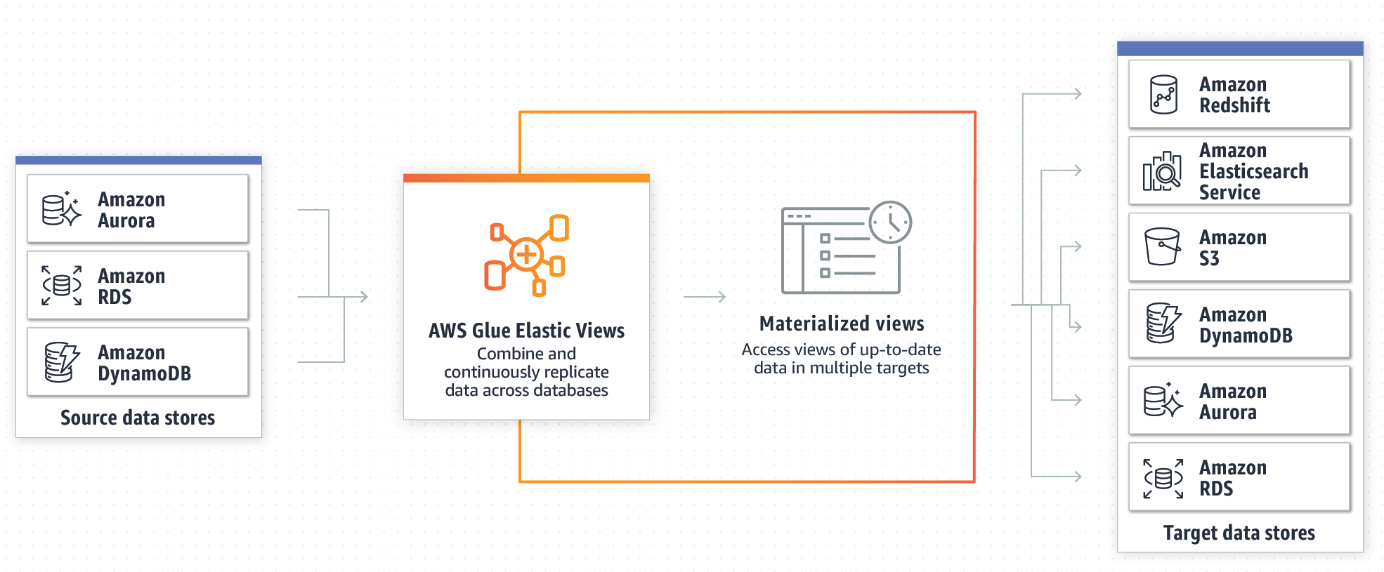
As shown in the image the focal point of this service is represented by the Materialized View, which is a way to abstract the dataset being it from any kind of data source: i.e. Amazon Aurora, RDS, or DynamoDB. This allows keeping things in synch without the actual use of a Glue Crawler as we would expect from our other articles about ETL workloads: for example this one, or this one.

But let’s take a look in detail at the main features and what they are useful for.

Use SQL as a mean to create a view

AWS Glue Elastic Views enables a developer to create materialized views across different data sources using SQL queries to aggregate the data. AWS Glue Elastic Views currently supports Amazon DynamoDB, Redshift, S3, and Elasticsearch Service. Also, AWS has plans to add even more data sources in the future.

Automatically copies data from the source data store to a target

AWS Glue Elastic Views manages the heavy lifting of copying and aggregating data from all the data sources to the target data stores, without having to write custom code or use complex or unfamiliar ETL tools and programming languages, having a beneficial effect on both time and efficiency of the project. AWS Glue Elastic Views reduces the time it takes to combine and replicate data across data stores from months to minutes according to AWS.

Keeps target’s data always up-to-date automatically

Keeping data in sync usually requires Crawlers and jobs to be created and maintained, AWS Glue Elastic Views, instead, continuously monitors for changes in data in the starting data stores, and when a change occurs, Elastic Views automatically updates the targets. This ensures that applications that access data using Elastic Views always have the most up-to-date data.

Alerts you if there is a change to the data model in a source data store

AWS Glue Elastic Views proactively alerts developers when there is a change to the data model in one of the source data stores so that they can update their views to adapt to this change.

Serverless

AWS Glue Elastic Views is serverless and scales capacity up or down automatically to accommodate workloads lifecycles. There is no hardware or software to manage, and as always, a user pays only for the resources it utilizes.

Register for the free preview

Being a service still in beta to try it it is necessary to register for the free preview: to do so, please go to this URL, and sign up, by compiling the form.

You’ll be asked for personal and company details, as well as a basic introduction to the business problem you want to solve using AWS Glue Elastic Views. Please be sure to give reasonable motivations, as interesting use cases increase the chances of being selected for the preview. 

Usually, AWS responds in a week, and if you are eligible for the preview the following message will be sent to your email.

After you have been registered, you’ll need to click on the AWS Glue Elastic View link in the email to access the service.

Now you’re ready to start your first ETL job with it, instead of using standard Spark scripts, or Glue Crawlers.

Our test case

The best way to understand the possibilities of this service is to try our hands on it. So we decided to create a simple use case to present how it could be used to enhance your ETL workloads.

Overview

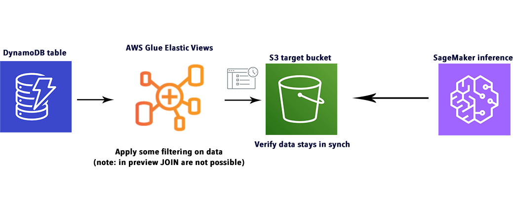
The basic idea is to populate a DynamoDB table with some test data obtained from free data sources. We want to extract and manipulate data from this table to demonstrate how Glue Elastic Views can effectively add ETL capabilities on top of DynamoDB, which is historically a little weak on this side. 

Then we want to send this data to S3 and verify that it is possible to update it in real-time to reflect changes, demonstrating how it can effectively speed up the investigation process of a Machine Learning pipeline.

Note: at the time of writing, unfortunately, JOIN operation is not supported for PartiQL in AWS Glue Elastic Views, so we opted for testing some mathematical and logical operations, as well as validating all the steps to synchronize the DynamoDB table with the S3 bucket.

Dataset

For our example, we decided to use a simple dataset about UFO sightings. We want to put this CSV file in a DynamoDB table, as stated before, and apply some filtering operations on latitude and longitude, or even city fields. The result will be used to answer the following example question: “How UFO sightings vary depending on different locations?”.

This is, of course, just a simple example, it has no practical meanings apart from demonstrating AWS Glue Elastic Views capabilities.

Import data in DynamoDB

We want to create the table for DynamoDB, to do that we’ve defined a simple script, in SageMaker Studio, to do the importing for us.

We basically read data from the CSV file using Pandas, we convert the rows to JSON, but before doing that we also add a “hash” column named id, because DynamoDB needs a primary key for each entry.

 for record in json_list:
        if record['longitude '] and record['latitude']:
    record['id'] = sha256(str(record).encode()).hexdigest()

The UFO dataset also had some problems that needed to be addressed: the “longitude” header had whitespace to be removed, and the latitude and longitude column needed to be converted in string removing NaN entries.

Finally, we used boto3 to create a corresponding table for the CSV.

dynamodb = boto3.resource('dynamodb')
table = dynamodb.Table('article_ufo_sightings')
with table.batch_writer() as batch:
...
batch.put_item(Item=record)

The complete code can be found here.

Note: we could have also used AWS Glue for this task, by putting the CSV file in a source S3 bucket using Glue Crawler to import data, but as we already covered ETL jobs with this service in other articles, we opted for a simpler solution as this is not the focus of the example.

Create DynamoDB table

We simply went to the DynamoDB console, clicked on “create table” and used these simple settings, just remember: apply on-demand capacity mode to speed up generating the table.

We add id as a primary key for UFO sightings. 

Creating Materialized View from table

Before generating the view, we needed to add the DynamoDB table as a source in AWS Glue Elastic Views; to do so, we went to the main console, selected “Tables” on the left, and clicked on “create table”. Then we just selected the new DynamoDB table from previous passages.

The next step was to apply some filtering in order to create our final target dataset, depending on the view. 

By going on the “Views” tab on the left side of the console we created a new one. Here we were presented with the ability to write custom PartiQL code: exactly what we wanted!

We added the following code in the editor to enable our Materialized View:

SELECT id, Latitude, Longitude FROM article_ufo_sightings.article_ufo_sightings

We also had to write all the attributes we wanted to export in the target parquet files (it seems that AWS Glue Elastic Views generates batches of parquet files in the output directory).

As the reader can see from the code above, we avoided requesting useful info on purpose: we want to show that it is possible to alter the view in real-time after the materialized view is created.

Send data to S3

At the time of writing, S3 is one of the three viable options for target along with ElasticSearch and Redshift, in our case S3 is the ideal target as we want the final dataset to be consumed by SageMaker. 

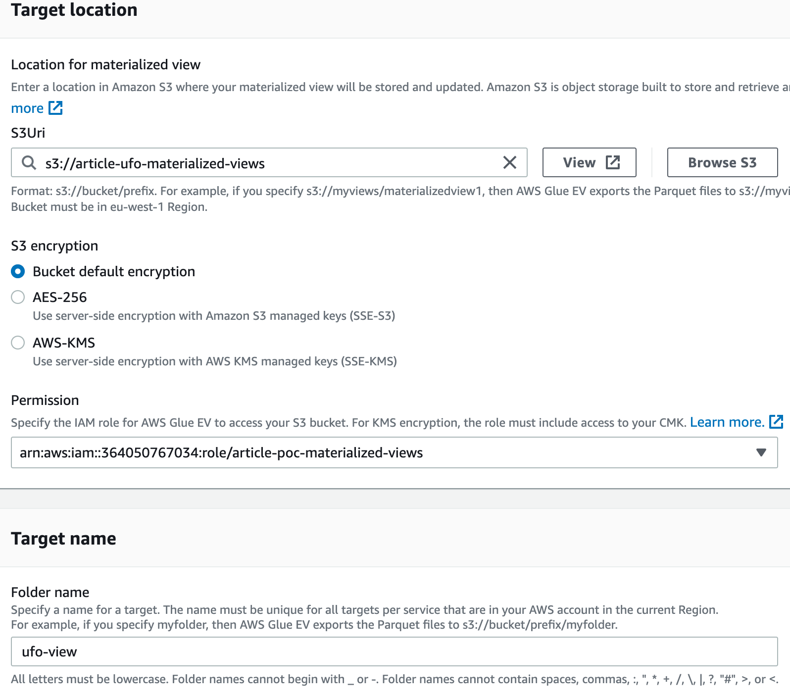
We went to the View and clicked on “Materialized View”, then we selected “Glue EV” as the support to unlock “S3” as a target: there we add the “article-ufo-materialized-views” bucket, we selected default encryption and we added a suitable IAM role for the execution. 

The role can be created using the AWS Role & Policy editor, then when the role is created, be aware to change the trust relationship with the code below to enable the IAM role, otherwise, you will not be able to see it in the selector:

  "Version": "2012-10-17",
  "Statement": [
    {
      "Effect": "Allow",
      "Principal": {
        "Service": [
          "materializedviews.amazonaws.com"
        ]
      },
      "Action": "sts:AssumeRole"
    }
  ]
}

Here is a screenshot with the settings we used:

When the view is created, it must be activated in order to synchronize with the S3 bucket, to do so, we went to both the table and the view we had created and clicked on “Activate” in their detail panel.

After a couple of minutes after activation, the S3 bucket was filled with the resulting data!

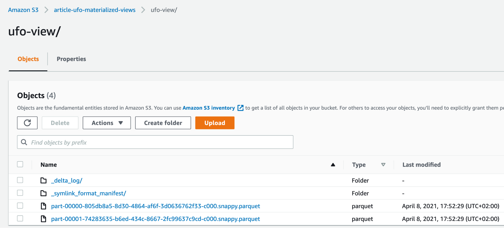
Interesting fact: just before activating the view, the service warned us that some fields were not compatible with the output target, and gave us the ability to modify the view on the fly with an inline editor, this is what we did to cast “Latitude” and “Longitude” fields to integer:

The data is now linked directly with our S3 bucket, so any change made to the table is reflected directly after some seconds. Basically is like having a Glue Crawler that works on-demand, going on and off when needed and without human intervention.

Alter the data on S3

We wanted to show that is possible to alter the data obtained from the DynamoDB table at any time, because of that, we started by saving “incomplete parquet files” as the reader can see here:

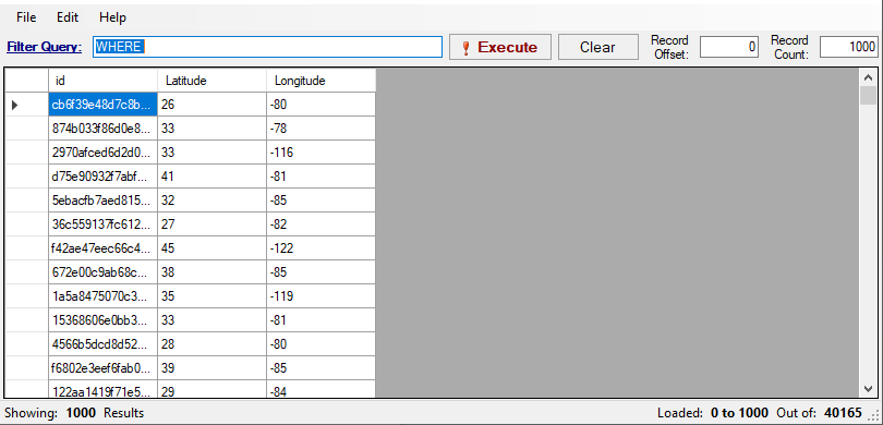
To modify our final dataset we first needed to “deactivate” the Materialized View. After that, it was possible to define a new Materialized view on the same target adding more columns. Please note also that, if you have more than one view depending on each other, you must deactivate and delete them in the correct order. Perhaps this operation will become less cumbersome by the time of the official release. 

We altered the original Materialized View definition adding more columns:

SELECT id,cast(City as string),cast(State as string),cast(Shape as string),cast(Latitude as integer),cast(Longitude as integer) FROM article_ufo_sightings.article_ufo_sightings;

Nonetheless, these operations took less than 5 minutes and the new data was soon ready in the correct S3 bucket:

Of course if the changes are on the original table and not on the view, updates are completely seamless as you would expect.

Another reminder: being the interface still in the preview phase, we recommend avoiding applying to many operations in a short time, as we experienced many bugs related to race conditions still not being managed correctly.

Make some Machine Learning out of it!

To test that the data source is viable for effective Machine Learning Jobs we’ve also prepared a simple SageMaker test notebook, to apply some correlation analysis on the created data lake. This can be seen in full detail in this notebook. The idea was to verify if there is some sort of correlation between locations, cities, and UFO sightings, and based on the example data, try to do some simple inferences. More info on how to use SageMaker to do inference was covered in this story.

References

• https://pages.awscloud.com/AWS-Glue-Elastic-Views-Preview.html
• https://aws.amazon.com/glue/features/elastic-views/
• https://aws.amazon.com/glue/faqs/
• https://cloudacademy.com/course/aws-reinvent-2020-aws-glue-elastic-views-1209/aws-glue-elastic-views/

Final Thoughts

We have reached the end of this journey into the wonders of AWS Elastic Views, so it’s time to sum up what we have learned so far.

This AWS Service proves itself to be invaluable when dealing with many different data sources, especially if of different nature, as it recovers and queries all the data with a SQL compatible language (PartiQL) avoiding the creation of many complex ETL Glue jobs.

It’s perfect in all those situations where you need to mix legacy and fresh data, as they usually reside, as per best practices, on different data sources: those cheaper for infrequent access and those with low latency for fresh data.

If you decide to use S3 as a target, it becomes a suitable solution for SageMaker Jobs or even managed tasks exploiting AWS Managed Machine Learning services.

If ElasticSearch is the designated target, Elastic Views becomes perfect for Business Intelligence workloads.

AWS Elastic Views support on-the-fly updates on data, with the ability to update even a single piece of data to reflect changes; all of this using simple, universally known, SQL language, bringing SQL capabilities for databases that don’t support it.

Being able to update a single field, avoid crawling again all the data in a data source to update the chosen target.

Finally, we would like to give advice though: as the current preview is still in a very early stage, most of the features described are not yet available to try, so even if the product is already useful in some cases, experiment before using it for production jobs, or wait for the public release.

So this is it! We hope you enjoyed the reading and gained useful insights. As always, feel free to comment in the section below, and reach us for any doubt, question or idea!

See you on #Proud2beCloud in a couple of weeks for another exciting story!