IoT ingestion and ML analytics pipeline with AWS IoT, Kinesis and SageMaker

Introduction

Machine Learning is rapidly becoming part of our daily life: it lets software and devices manage routines without human intervention and moreover gives us the ability to automate, standardize, and simplify many daily tasks. One interesting topic is, for example, home automation, where it is now possible to have intelligent lights, smart heating, and autonomous robots that clean floors even in complex home landscapes filled with obstacles. 

Generally speaking, information retrievable from connected devices is nearly infinite. Cheap cost of data acquisition, and computational power to manage big data, made Machine Learning accessible to many use-cases. One of the most interesting is ingestion and real-time analysis of IoT connected devices.

In this article, we would like to share a solution that takes advantage of AWS Managed Services to handle high volumes of data in real-time coming from one or more IoT connected devices. We’ll show in detail how to set up a pipeline to give access to potential users to near real-time forecasting results based on the received IoT data. 

The solution will also explore some key concepts related to Machine Learning, ETL jobs, Data Cleaning, and data lake preparation.

But before jumping into code and infrastructure design, a little  recap on ML, IoT, and ETL is needed. Let’s dive together into it!

IoT, Machine Learning and Data Transformation: key concepts

IoT

The Internet of things (IoT) is a common way to describe a set of interconnected physical devices — “things” — fitted with sensors, that to  exchange data to each other and over the Internet.

IoT has evolved rapidly due to the decreasing cost of smart sensors, and to the convergence of multiple technologies like real-time analytics, machine learning, and embedded systems.

Of course, traditional fields of embedded systems, wireless sensor networks, control systems, and automation, also  contribute to the IoT world.

Machine Learning

ML was born as an evolution of Artificial Intelligence . Traditional ML required the programmers to write complex and difficult to maintain heuristics in order to carry out a traditionally human task (e.g. text recognition in images) using a computer.

With Machine Learning it is the system itself that learns relationships between data.

For example, in a chess game, there is no longer an algorithm that makes chess play, but by providing a dataset of features concerning chess games, the model learns to play by itself. 

Machine Learning also makes sense in a distributed context where the prediction must scale.

Data Transformation

In a Machine Learning pipeline, the data must be uniform, i.e. standardized. Differences in the data can result from heterogeneous sources, such as different DB table schema, or different data ingestion workflows . 

Transformation (ETL: Extract, transform, load) of data is thus an essential step  in all ML pipelines. Standardized data are not only essential in training the ML model but are also much easier to analyse and visualize in the preliminary data discovery step.

In general, for data cleaning and formatting, Scipy Pandas and similar libraries are usually used.

- NumPy:  - library for the management of multidimensional arrays, it is mainly used in the importing and reading phase of a dataset.

- Pandas Dataframe: - library for managing data in table format. It takes data points from CSV, JSON, Excel, and pickle files and transforms them into tables. 

- SciKit-Learn: - library for final data manipulation and training.
Cleaning and formatting the data is essential to ensure the best chance for the model to converge well to the desired solution.

The Pipeline

To achieve our result, we will make extensive use of what AWS gives us in terms of managed services. Here is a simple sketch, showing the main actors involved in our Machine Learning pipeline.

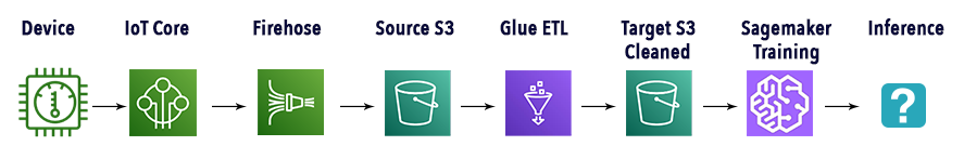
Let’s see take a look at the purpose of each component before going into the details of each one of them.

The pipeline is organized into 5 main phases: ingestion, datalake preparation, transformation, training, inference.

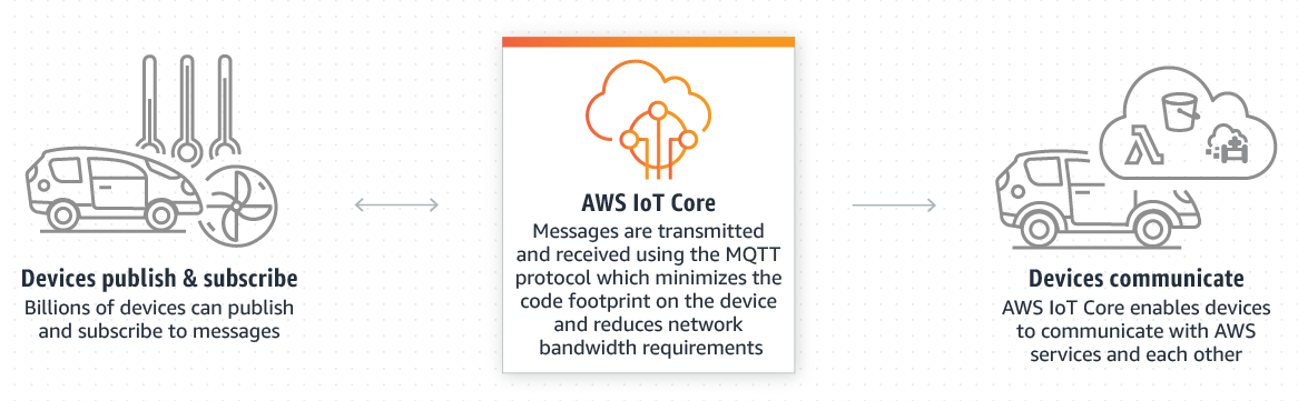
The ingestion phase will receive data from our connected devices using AWS IoT Core to allow connecting them with AWS services without managing servers and communication complexities. Data  from the devices will be sent  using the MQTT protocol to minimize code footprint and network bandwidth. Should you need it AWS IoT Core can also manage device authentication.

To send information to our Amazon S3 data lake we will use Amazon Kinesis Data Firehose which comes with a built-in action for reading AWS IoT Core messages.
To transform data and make it available for Amazon SageMaker we will use AWS Glue: a serverless data integration service that makes it easy to find, prepare and combine data for analytics, machine learning, and application development. AWS Glue provides all the capabilities needed for data integration, to start analyzing and using data in minutes rather than months.

Finally, to train and then deploy our model for online inference we will show how to leverage built-in algorithms from Amazon SageMaker, in particular, DeepAR.

Ingestion: AWS IoT Core to Amazon Kinesis Data Firehose

To connect our test device to AWS we used AWS IoT Core capabilities. In the following, we assume that the reader already has an AWS account ready. 

AWS IoT Core

Go to your account and then search for “IoT Core” then in the service page, in the sidebar menu, choose “Get started” and then select “Onboard a device”. 

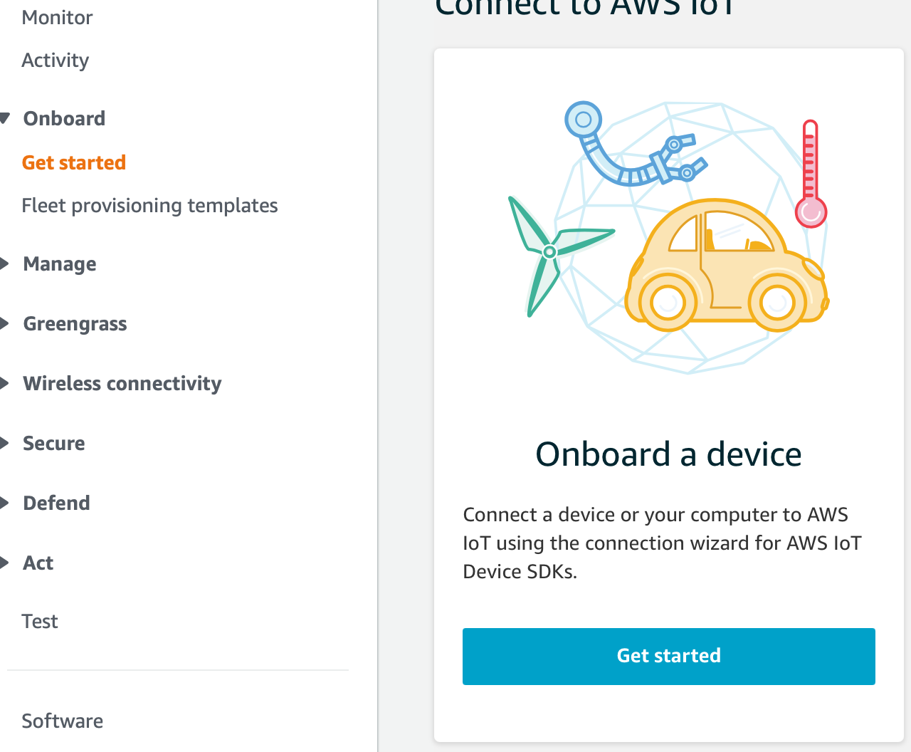
Follow the wizard to connect a device as we did. The purpose is to:

1. Create an AWS IoT Thing
2. Download the requested code directly to your device to allow connection to AWS.

This is important because we also connect Amazon Kinesis Data Firehose to read the messages sent from AWS IoT Core. As a side note, remember that you need access to the device and that device must have a TCP connection to the public internet on port 8883.

Following the wizard, select Linux as the OS and an SDK (in our case Node.js):

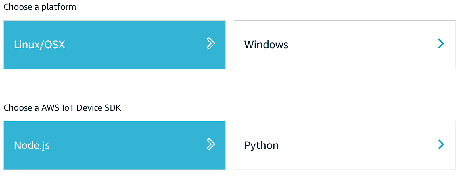
After that, we gave a name to the new “thing” and got the connection kit which contains:

• The SDK selected
• An example program
• The certificates necessary to connect the device

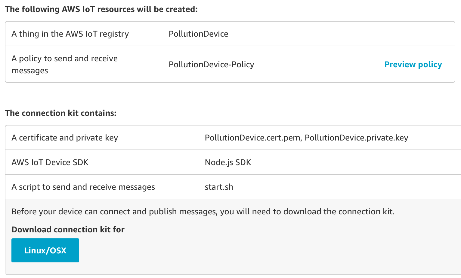
Once downloaded, initialize a new Node.js project and install AWS-IoT-device-SDK. This will install the required node modules; after that, it is possible to run the included start.sh script, by including all the certificates downloaded with the kit in the same project directory.
We developed our example using device-example.js as a simple base to understand how to connect a device to AWS IoT.

const deviceModule = require('aws-iot-device-sdk').device;
const cmdLineProcess = require('aws-iot-device-sdk/examples/lib/cmdline');
processPollutionData = (args) => {
   // Device properties which are needed
   const device = deviceModule({
       keyPath: args.privateKey,
       certPath: args.clientCert,
       caPath: args.caCert,
       clientId: args.clientId,
       region: args.region,
       baseReconnectTimeMs: args.baseReconnectTimeMs,
       keepalive: args.keepAlive,
       protocol: args.Protocol,
       port: args.Port,
       host: args.Host,
       debug: args.Debug
   });
   const minimumDelay = 250; // ms
   const interval = Math.max(args.delay, minimumDelay);
   // Send device information
   setInterval(function() {
       // Prepare Data to be sent by the device
       const payload = {
           ozone: Math.round(Math.random() * 100),
           particullate_matter: Math.round(Math.random() * 100),
           carbon_monoxide: Math.round(Math.random() * 100),
           sulfure_dioxide: Math.round(Math.random() * 100),
           nitrogen_dioxide: Math.round(Math.random() * 100),
           longitude: 10.250786139881143,
           latitude: 56.20251117218925,
           timestamp: new Date()
       };
       device.publish('', JSON.stringify(payload));
   }, interval);
   // Device callbacks, for the purpose of this example we have put
   // some simple console logs
   device.on('connect', () => { console.log('connect'); });
   device.on('close', () => { console.log('close'); });
   device.on('reconnect', () => { console.log('reconnect'); });
   device.on('offline', () => { console.log('offline'); });
   device.on('error', (error) => { console.log('error', error); });
   device.on('message', (topic, payload) => { 
console.log('message', topic, payload.toString()); 
   });
}
// this is a precooked module from aws to launch
// the script with arguments
module.exports = cmdLineProcess;
// Start App
if (require.main === module) {
   cmdLineProcess('connect to the AWS IoT service using MQTT',
       process.argv.slice(2), processPollutionData);
}

We required the Node.js modules necessary to connect the device to AWS and to publish to a relevant topic. You can read data from your sensor in any way you want, for example, if the device can write sensor data in a specific location, just read and stringify that data using device.publish('<YOUR_TOPIC>', JSON.stringify(payload)).

The last part of the code just calls the main function to start sending information to the console.

To run the script use the start.sh script included in the development kit, be sure to point to your code and not the example one from AWS. Leave the certificates and client ID as they are because they were generated from your previous setup.

Note: for the sake of this article the device code is oversimplified, don’t use it like this in production environments.

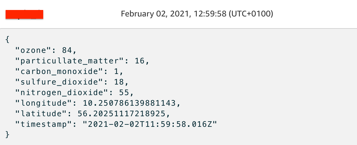
To test that everything is working as intended, access the AWS IoT console, go to the Test section in the left sidebar and when asked, type the name of your topic and click “Subscribe to topic”. If everything is set up correctly you should see something like the screenshot below:

Now we need to connect Amazon Kinesis Data Firehose to start sending data to Amazon S3.

Amazon Kinesis Data Firehose

Keeping the data lake up to date populate the data lake with the data sent by the device, is extremely important to avoid a problem called Concept Drift which happens when there is a gradual misalignment of the deployed model with respect to the world of real data; this happens because the historical data can no longer represent the problem that has evolved. 

To overcome this problem we must ensure efficient logging and the means to understand when to intervene on the model e.g. by retraining or upgrading the version and redeploy the updated version. To help with this kind of “problem” we define Amazon Kinesis Data Firehose action, specifically to automatically register and transport every MQTT message delivered from the device, directly to Amazon S3 to provide our data lake always with fresh data.

Create the Firehose stream

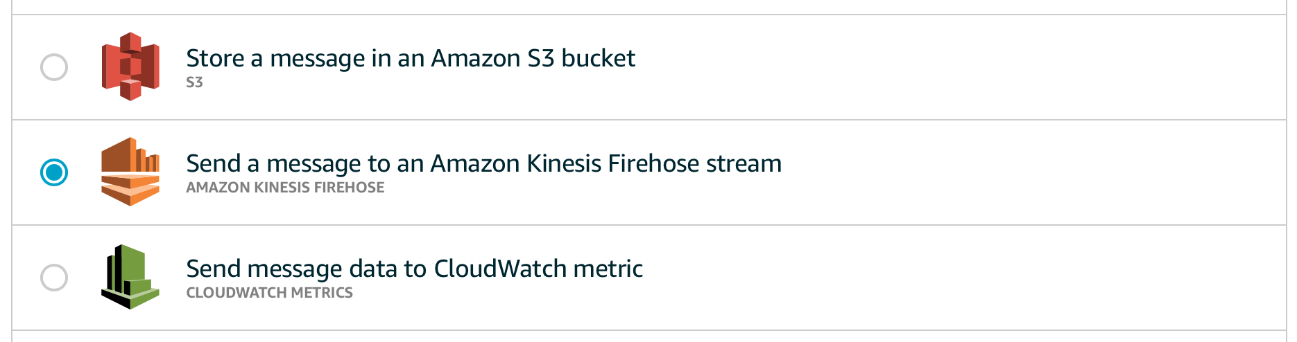
To create a Firehose stream search for “Kinesis firehose” in the service search bar, select it, then “Create delivery stream” like in the figure:

Select a valid name, under “Delivery stream name”, “Direct PUT or other sources” under “Sources”, and then, on the next page, leave everything as it is (we will convert data in Amazon S3 later), finally in the last page select Amazon S3 as a destination and eventually add a prefix to the data inserted in the bucket. Click “Next” and create the stream.

Create the IoT Rule

To use the stream we must connect it with AWS IoT by the means of an IoT Rule; this rule will allow Amazon Kinesis Data Firehose to receive messages and write them to an Amazon S3 bucket. To configure AWS IoT to send to Firehose we followed these steps:.

1. When creating a rule in the AWS IoT console, on the Create a rule page, under Set one or more actions, choose “Add action”.
2. Choose “Send a message to an Amazon Kinesis Firehose stream”.

3. Choose “Configure action”.
4. For the Stream name, choose the Amazon Kinesis Data Firehose delivery stream we’ve just created.
5. For Separator, choose a separator character to be inserted between records for example comma (,).
6. For the IAM role name, choose “Create a new role”.
7. Choose “Add action”.

This is an example of how such a rule will then be created:

{
    "topicRulePayload": {
        "sql": "SELECT * FROM ''", 
        "ruleDisabled": false, 
        "awsIotSqlVersion": "2016-03-23",
        "actions": [
            {
                "firehose": {
                    "deliveryStreamName": "",
                    "roleArn": "arn:aws:iam:::role/"
                }
            }
        ] 
    }
}

If everything is ok, you’ll start seeing data showing in your bucket soon, like in the example below:

And opening one of these will show the data generated from our device!

Datalake: Amazon S3

Amazon Simple Storage Service is an object storage service ideal for building a datalake. With almost unlimited scalability, an Amazon S3 datalake provides many benefits when developing analytics for Big Data. 

The centralized data architecture of Amazon S3 makes it simple to build a multi-tenant environment where multiple users can bring their own Big Data analytics tool to analyze a common set of data. 

Moreover, Amazon S3 integrates seamlessly with other Amazon Web Services such as Amazon Athena, Amazon Redshift, and like in the case presented, AWS Glue. 

Amazon S3 also enables storage to be decoupled from compute and data processing to optimize costs and data processing workflows, as well as to keep the solution dry, scalable, and maintainable.

Additionally, Amazon S3 allows you to store any type of structured, semi-structured, or even unstructured data in its native format. In our case, we are simply interested in saving mocked data from a test device to make some simple forecasting predictions. 

ETL process: AWS Glue

Even if the data is saved on Amazon S3 on a near-real time basis, it is still not enough to allow us  to train an Amazon SageMaker model. As we explained in the introduction in fact the data must be prepared and when dealing with predefined Amazon SageMaker algorithms some defaults must be kept in mind.

For example, Amazon SageMaker doesn’t accept headers, and in case we want to define a supervised training, we also need to put the ground truth as the first column of the dataset.

In this simple example we used AWS Glue studio to transform the raw data in the input Amazon S3 bucket to structured parquet files to be saved in a dedicated output Bucket. The output bucket will be used by Amazon Sagemaker as the data source.

AWS Glue Crawler

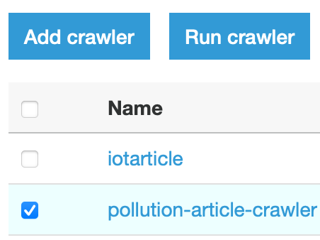
At first, we need a Crawler to read from the source bucket to generate an AWS Glue Schema. To create it go to the AWS Glue page, select Crawlers under “Glue console”, add a new crawler, by simply giving a name, selecting the source Amazon S3 bucket and the root folder created by Amazon Kinesis Data Firehose. A new schema will be created from this information. Leave all other options as default.

Activate the Crawler once created, by clicking on “Run crawler”.

The next step is to set up an AWS Glue Studio job using the Catalog as the data source..

ETL job

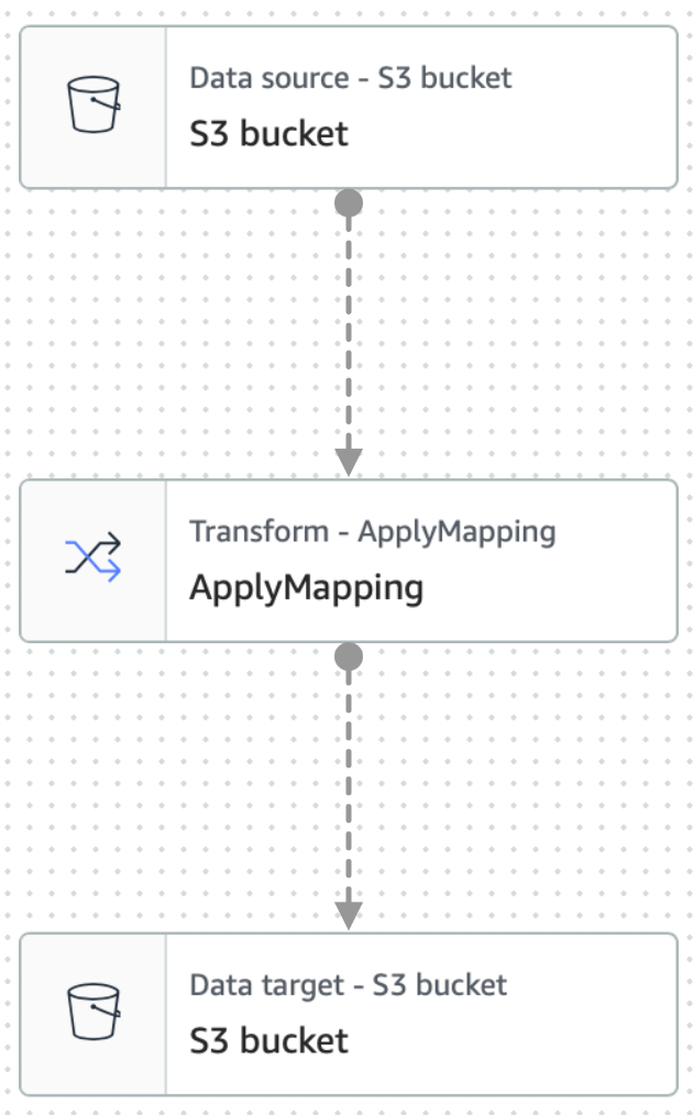
An AWS Glue Studio job consists of at least 3 main nodes, which are source, transform, and target. We need to configure all three nodes to define a crawler capable of reading and transforming data on the fly.

To do so, here are the step we followed:

1. Choose Create and manage jobs from AWS Glue Studio dashboard.
2. On the Manage Jobs page, choose the source and target added to the graph option. Then, choose Amazon S3 for the Source and Amazon S3 for the Target.

3. Click the Create button to start the job creation process.

Now you’ll see a  three-node graph displayed that represents the steps involved in the ETL process. When AWS Glue is instructed to read from an Amazon S3 data source, it will also create an internal schema, called Glue Data Catalog.

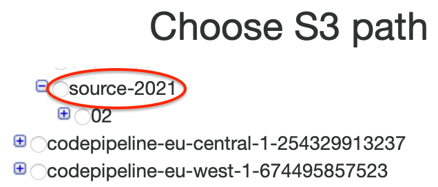
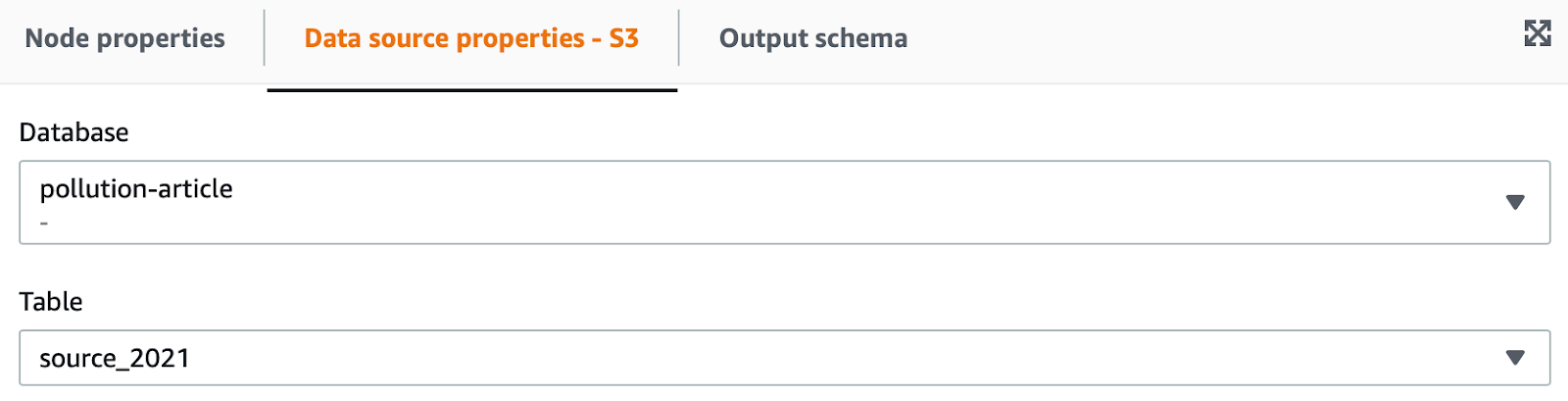
To configure the source node, click on it in the graph:

1. On the Node Properties tab, for Name, enter a name that is unique for this job. The value you enter is used as the label for the data source node in the graph. Choose the Data source properties - Amazon S3 tab in the node details panel.
2. Select your crawler database from the list of available databases in the AWS Glue Data Catalog.
3. Choose the correct table from the Catalog.

The same can be done for the transform node: by clicking on it is possible to define what kind of transformation we want to apply to input data. Here you can also verify that the JSON data is imported correctly:

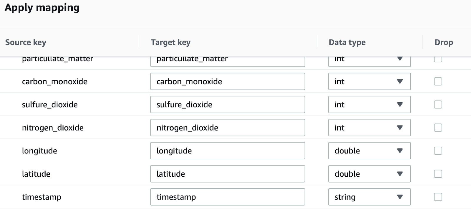
Finally, we can select the target node, specifying, again Amazon S3 as a target, and using .parquet as the output format.

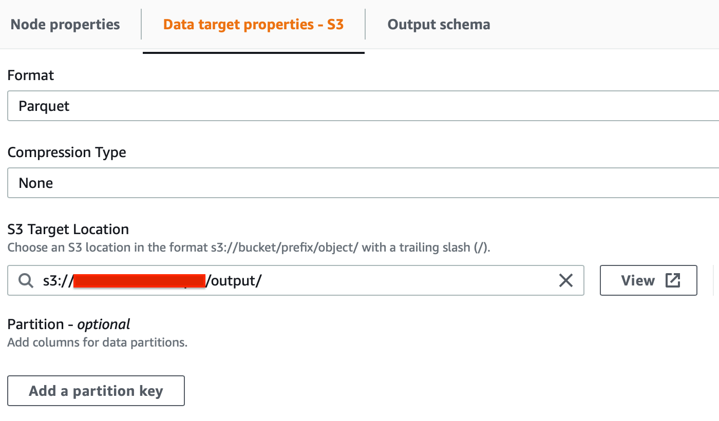
Now we need to set the ETL job parameters for the workflow just created. Go to the “Job details” tab on the right, give a name, and select a role capable of managing data and deploying again on Amazon S3. 

Leave the rest as default. 

Note that you must have this snippet on the “Trust Relationship” tab of the role to let it assume be assumed by AWS Glue:

{ 
    "Version": "2012-10-17", 
    "Statement": [ 
       { 
          "Effect": "Allow", 
          "Principal": { "Service": "glue.amazonaws.com" }, 
          "Action": "sts:AssumeRole" 
       } 
    ]
}

If everything is defined correctly, the job will start and begin converting your data in parquet format. The files will be put in your out directory in the bucket of your choice.

Dataset optimization: why parquet over CSV

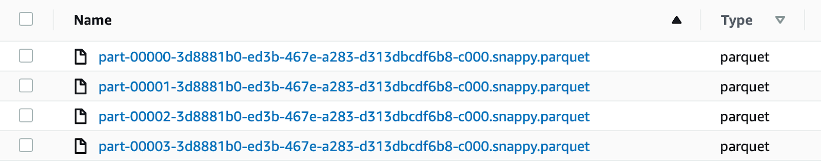
We chose to use parquet instead of the CSV data format for the target dataset. Parquet is a highly compressed columnar format, which uses the record shredding and assembly algorithm, vastly superior to the simple flattening of nested namespaces. It has the following advantages:

• It brings efficiency compared to row-based files like CSV. When querying, columnar storage skipping non-relevant data can be done very quickly. 

• Aggregation queries are less time-consuming compared to row-oriented databases, minimizing latency for accessing data.

• Apache Parquet can support advanced nested data structures. 

• Parquet is built to support flexible compression options and efficient encoding schemes. 

• Apache Parquet works best with interactive and serverless technologies like AWS Athena, Amazon Redshift, and AWS Glue.

Also compared to file stored in .csv format we have these advantages in terms of cost savings:

• Amazon Athena and Redshift Spectrum will charge based on the amount of data scanned per query.
• Amazon charges according to the amount of data stored on Amazon S3.
  

The Machine Learning step: Forecasting with Amazon SageMaker

Amazon SageMaker offers 17 prebuilt algorithms out-of-the-box that cover a plethora of topics related to Machine Learning problems. In our case, we wanted to simplify the development of a forecasting model for the data retrieved from our device, so instead of showing how to bring your own algorithm, like in our previous article, this time we’ll be using a pre-cooked one.

As explained before, apart from cleaning data, our ETL process was done to transform the data to be compatible with ready-made Amazon SageMaker algorithms.

Amazon SageMaker API and Sklearn Library offer methods to retrieve the data, call the training method, save the model, and deploy it to production for online or batch inference.

Start by going to the Amazon SageMaker page and creating a new notebook instance, for this article we chose an ml.t3.medium. Add a name and create a new IAM role.

Leave the rest as default and click “Create notebook”.

Access it by either Jupiter or Jupiter Lab, we chose the second. We managed to put up a simple notebook illustrating all the steps involved in using the pre-backed DeepAR algorithm by Amazon Sagemaker. 

Note: the code is made solely for this article and is not meant for production as there is no preliminary investigation on data and no validation of the results. Still, all the code presented is tested and usable for use cases similar to the one presented.

We start by importing all the necessary libraries:

import time
import io
import math
import random
import numpy as np
import pandas as pd
import JSON
import matplotlib.pyplot as plt
import boto3
import sagemaker
from sagemaker import get_execution_role

# set random seeds for reproducibility
np.random.seed(42)
random.seed(42)

We also set the seed for our random methods to ensure reproducibility. After that, we need to recover our parquet files from Amazon S3 and obtain a Pandas Dataframe from them.

bucket = ""
data = "output"
model = "model"
sagemaker_session = sagemaker.Session()
role = get_execution_role()
s3_data_path = f"{bucket}/{data}"
s3_output_path = f"{bucket}/{model}/"

At first, we prepare all the Amazon S3 “paths” that will be used in the notebook, and we generate an Amazon SageMaker Session and a valid IAM Role with get_execution_role(). As you can see Amazon SageMaker takes care of all these aspects for us.

from sagemaker.amazon.amazon_estimator import get_image_uri
image_uri = get_image_uri(boto3.Session().region_name, "forecasting-deepar")

In the step above we recover our forecasting Estimator, DeepAR. An estimator is a class in Amazon SageMaker capable of generating, and testing a model which will then be saved on Amazon S3.

Before starting to read the parquet files we also add a couple of constants to our experiment:

freq = "H"
prediction_length = 24
context_length = 24 # usually prediction and context are set equal or similar

With freq (frequency) we say that we want to analyze the TimeSeries by hourly metrics. Prediction and Context length are set to 1 day and they are respectively how many hours we want to predict in the future and how many in the past we’ll use for the prediction. Usually, these values are defined in terms of days as the dataset is much bigger.

We created two helper methods to read from parquet files:

# Read single parquet file from S3
def pd_read_s3_parquet(key, bucket, s3_client=None, **args):
    if not s3_client:
        s3_client = boto3.client('s3')
    obj = s3_client.get_object(Bucket=bucket, Key=key)
    return pd.read_parquet(io.BytesIO(obj['Body'].read()), **args)

# Read multiple parquets from a folder on S3 generated by spark
def pd_read_s3_multiple_parquets(filepath, bucket, **args):
    if not filepath.endswith('/'):
        filepath = filepath + '/'  # Add '/' to the end
    
    s3_client = boto3.client('s3')   
    s3 = boto3.resource('s3')
    s3_keys = [item.key for item in s3.Bucket(bucket).objects.filter(Prefix=filepath)
               if item.key.endswith('.parquet')]
    if not s3_keys:
        print('No parquet found in', bucket, filepath)
    
    dfs = [pd_read_s3_parquet(key, bucket=bucket, s3_client=s3_client, **args) 
           for key in s3_keys]
    return pd.concat(dfs, ignore_index=True)

Then we actually read the datasets:

# get all retrieved parquet in a single dataframe with helpers functions
df = pd_read_s3_multiple_parquets(data, bucket)
df = df.iloc[:, :8] # get only relevant columns
df['hour'] = pd.to_datetime(df['timestamp']).dt.hour #add hour column for the timeseries format
# split in test and training
msk = np.random.rand(len(df)) < 0.8 # 80% mask
# Dividing in test and training
training_df = df[msk]
test_df = df[~msk]

Here we manipulate the dataset to make it usable with DeepAR which has its proprietary input format. We use df.iloc[:, :8] to keep only the original columns without the ones produced by AWS Glue Schema. We generate a new hour column to speed things up, finally, we split the dataset in 80/20 proportion for training and testing.

We then write back data to Amazon S3 temporarily as required by DeepAR, by building JSON files with series in them.

# We need to resave our data in JSON because this is how DeepAR works
# Note: we know this is redundant but is for the article to show how many ways 
# there are to transform dataset back and forth from when data is acquired

train_key = 'deepar_training.json'
test_key  = 'deepar_test.json'

# Write data in DeepAR format
def writeDataset(filename, data): 
    file=open(filename,'w')
    previous_hour = -1
    for hour in data['hour']:
        if not math.isnan(hour):
            if hour != previous_hour:
                previous_hour = hour
                # One JSON sample per line
                line = f"\"start\":\"2021-02-05 {int(hour)}:00:00\",\"target\":{data[data['hour'] == hour]['ozone'].values.tolist()}"
                file.write('{'+line+'}\n')

The generated JSON documents  are structured in a format like this:

{"start":"2021-02-05 13:00:00","target":[69.0, 56.0, 2.0, …]}

After that, we can write our JSON files to Amazon S3.

writeDataset(train_key, training_df)        
writeDataset(test_key, test_df)

train_prefix   = 'model/train'
test_prefix    = 'model/test'

train_path = sagemaker_session.upload_data(train_key, bucket=bucket, key_prefix=train_prefix)
test_path  = sagemaker_session.upload_data(test_key,  bucket=bucket, key_prefix=test_prefix)

We use sagemaker_session.upload_data() for that, passing the output location. Now we can finally define the estimator:

estimator = sagemaker.estimator.Estimator(
    sagemaker_session=sagemaker_session,
    image_uri=image_uri,
    role=role,
    instance_count=1,
    instance_type="ml.c4.xlarge",
    base_job_name="pollution-deepar",
    output_path=f"s3://{s3_output_path}",
)

We’ll pass the Amazon SageMaker session, the algorithm image, the instance type, and the model output path to the estimator. We also need to configure some Hyperparameters:

hyperparameters = {
    "time_freq": freq,
    "context_length": str(context_length),
    "prediction_length": str(prediction_length),
    "num_cells": "40",
    "num_layers": "3",
    "likelihood": "gaussian",
    "epochs": "20",
    "mini_batch_size": "32",
    "learning_rate": "0.001",
    "dropout_rate": "0.05",
    "early_stopping_patience": "10",
}

estimator.set_hyperparameters(**hyperparameters)

These values are taken directly from the official AWS examples on DeepAR. We also need to pass the two channels, training, and test, to the estimator to start the fitting process.

data_channels = {"train": train_path, "test": test_path}
estimator.fit(inputs=data_channels)

After training and testing a model, we can deploy it using a Real-time Predictor.

# Deploy for real time prediction
job_name = estimator.latest_training_job.name

endpoint_name = sagemaker_session.endpoint_from_job(
    job_name=job_name,
    initial_instance_count=1,
    instance_type='ml.m4.xlarge',
    role=role
)

predictor = sagemaker.predictor.RealTimePredictor(
    endpoint_name, 
    sagemaker_session=sagemaker_session, 
    content_type="application/json")

The predictor generates an endpoint that is visible from the AWS console.

The endpoint can be called by any REST enabled application passing a request with a format like the one below:

{
  "instances": [ 
    {
       "start": "2021-02-05 00:00:00",
       "target": [88.3, 85.4, ...]
    }
  ],
  "configuration": {
    "output_types": ["mean", "quantiles", "samples"],
    "quantiles": ["0.1", "0.9"], 
    "num_samples": 100
  }
}

The “targets” are some sample values starting from the period set in “start” by which we want to generate the prediction.

Finally, if we don’t need the endpoint anymore, we can delete it with:

sagemaker_session.delete_endpoint(endpoint_name)

Real-Time Inference: from concept to production

Real-time inference refers to the prediction given in real-time by some models. This is the typical use case of many recommendation systems or generally when the prediction concerns a single-use. It is used when:

• We are dealing with dynamic data.
• We have low-latency required.
• We want real-time predictions.
• It is characterized by a single prediction.

 It's typically a bit more complex to manage compared to what we have done in the notebook and is typically defined in a separate pipeline, due to its nature of high availability and fast response time.

When deploying using Amazon SageMaker API it is possible to create a deploy process that is very similar to how a web application is deployed or upgraded, taking into account things like traffic rerouting and deploy techniques like Blue/Green or Canary. We want to share with you a summary guide for both methods so that you can try them by yourself!

How to deploy

1. Create a model using CreateModelApi.
2. Create an HTTPS endpoint using CreateEndpointConfigApi entering as properties:
   
   • The model
   • The production variants
   • Instance type
   • Instance count
   • Weight

3. Finalize the creation of the endpoint using CreateEndpointApi.Pass the data of the two previous configurations and any tags to this last command.

Note: through the production variants we can implement different Deploy strategies such as A/B and BLUE/GREEN.

Deploy Blue / Green

1. Create a new version of the model.
2. Create an endpoint configuration by copying the data from the old one.
3. Update the production variants by adding the new configuration.
4. Call UpdateEndpointApi with the new configuration. The Green infrastructure is added, here’s where we can do synthetic testing.
5. Redirect traffic to Green. If Green performs well, with another UpdateEndpointApi delete the old model.

Deploy A / B

To be used if we want to measure the performance of different models with respect to a high-level metric.

1. Create multiple models using the same configuration.
2. Update or create a Configuration by modifying or creating the production variants.
3. Set the balancing weights to 50/50.
4. Check functionality and performance.
5. Gradually change the % of traffic.

In the end, exclude one or more models.

Note: the multi-model for endpoint property allows for managing multiple models at the same time, the machine memory is managed automatically based on the traffic. This approach can save money through the optimized use of resources.

References

• https://docs.aws.amazon.com/iot/latest/developerguide/iot-quick-start.html
• https://docs.aws.amazon.com/iot/latest/developerguide/kinesis-firehose-rule-action.html
• https://docs.aws.amazon.com/glue/latest/ug/tutorial-create-job.html
• https://docs.aws.amazon.com/iot/latest/developerguide/topics.html
• https://docs.aws.amazon.com/AmazonCloudWatch/latest/monitoring/CloudWatch_Synthetics_Canaries.html
• https://mqtt.org/
• https://machinelearningmastery.com/gentle-introduction-concept-drift-machine-learning/
• https://parquet.apache.org/

Takeaways 

In this article, we have seen how to develop a pipeline using AWS resources to ingest data from a device connected to the AWS ecosystem through AWS IoT Core. 

We have also seen how to efficiently read and store data as it is sent by the devices using Amazon Kinesis Data Firehose, acting as a near real-time stream, to populate and update our data lake on Amazon S3.

To perform the needed ETL data transformation we chose AWS Glue Studio, showing how easily it can be configured to create a crawler to read, transform, and put data back to Amazon S3, ready to be used for model training.

We then explained why using the parquet format is better than a simple CSV format. In particular, we focused on the performance improvement with respect to CSV for import/export, Athena query operations and how much more convenient is the pricing on Amazon S3 due to a significantly smaller file size.

Amazon SageMaker can be used out-of-the-box with its set of prebuilt algorithms and in particular, we’ve seen how to implement a forecasting model on our mocked dataset consisting of environmental and pollution data.

Finally, we put the model into production, leveraging Amazon SageMaker APIs to create a deploy pipeline that takes into account the Concept Drift problem, thus allowing for frequent updates of the model based on the evolution of the dataset in time. This is especially true for time-series and forecasting models, which become better and better as the dataset grows bigger. 

We are at the end of the journey for this week!. As always feel free to comment and give us your opinions and ideas. What about your use-cases? What kind of devices do you use? Reach us and talk about it!

We are at the end of the journey for this week!. As always feel free to comment and to give us your opinions and ideas. What about your use-cases? What kind of devices do you use? Reach us and talk about it!
Stay tuned and see you in 14 days on #Proud2BeCloud!

About beSharp

Proud2beCloud is a blog by beSharp, an Italian APN Premier Consulting Partner expert in designing, implementing, and managing complex Cloud infrastructures and advanced services on AWS. Before being writers, we are Cloud Experts working daily with AWS services since 2007. We are hungry readers, innovative builders, and gem-seekers. On Proud2beCloud, we regularly share our best AWS pro tips, configuration insights, in-depth news, tips&tricks, how-tos, and many other resources. Take part in the discussion!