Orchestrating Data Analytics and Business Intelligence pipelines via AWS Step Functions

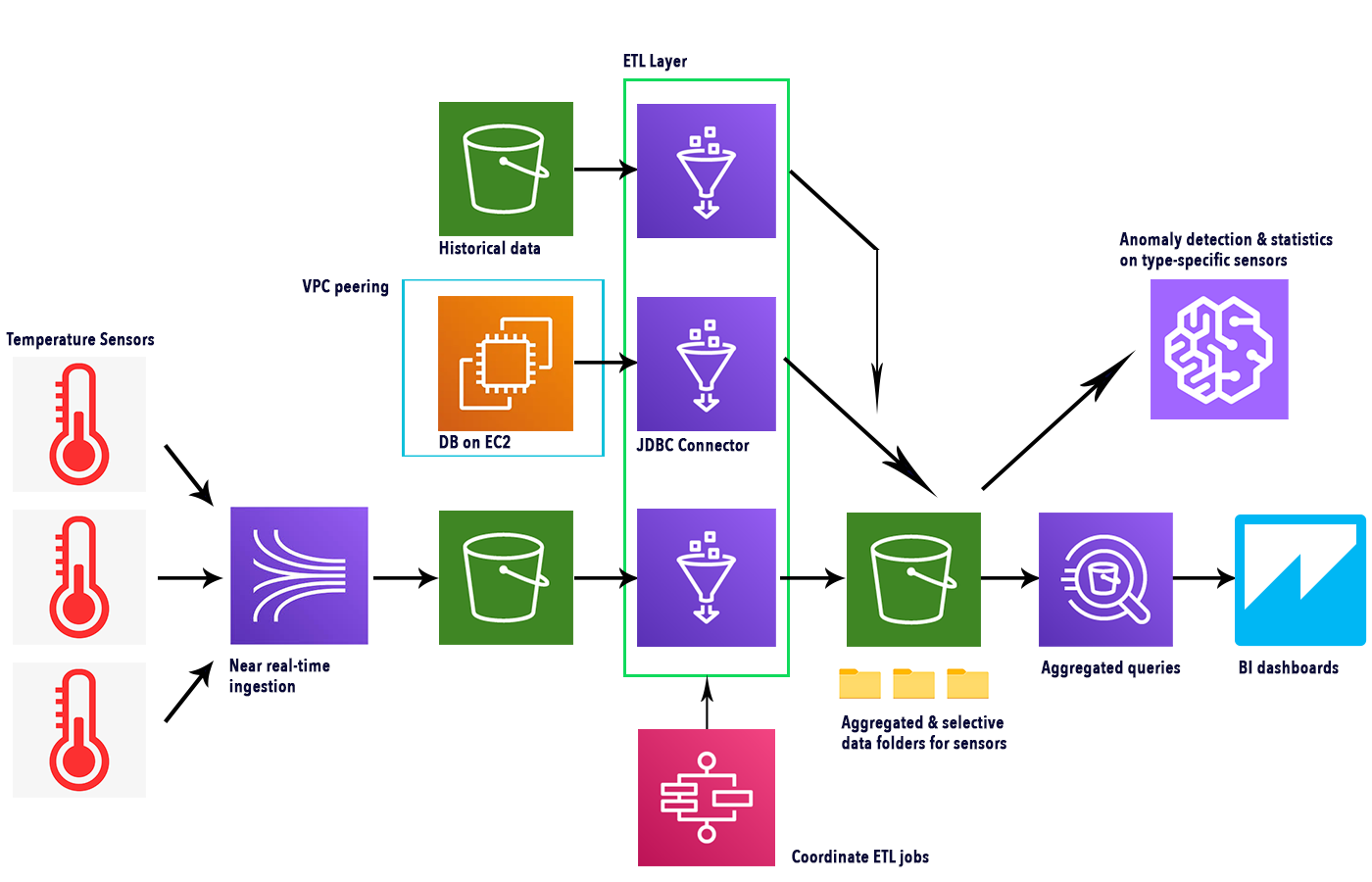
ETL pipelines on AWS usually have a linear behavior: starting from one service and ending to another one. This time though, we would like to present a more flexible setup, in which some ETL jobs could be skipped depending on data. Furthermore, some of the transformed data in our data lake need to be queried by AWS Athena in order to generate BI dashboards in QuickSight while other data partitions are used to train ad-hoc anomaly detection via Sagemaker.

A powerful tool to orchestrate this type of ETL pipelines is the AWS StepFunctions service.

In this article, we want to show you some of the steps involved in the creation of the pipeline as well as how many AWS services for data analytics can be used in near real-time scenarios to manage a high volume of data in a scalable way.

In particular, we’ll investigate AWS Glue connectors and Crawlers, AWS Athena, QuickSight, Kinesis Data Firehose, and finally a brief explanation on how to use of SageMaker to create forecasts starting from the collected data. To learn more about Sagemaker you can also take a look at our other articles.

Let’s start!

Our setup

In this example, we’ll set up several temperature sensors to send temperature and diagnostic data to our pipeline and we’ll perform different BI analyses to verify efficiency, and we’ll use a Sagemaker model to check for anomalies.

To keep things interesting we also want to grab historical data from two different locations: an S3 bucket and a Database residing on an EC2 instance in a different VPC from one of our ETL pipelines.

We will use different ETL jobs to recover and extract cleaned data from row data and AWS Step Functions to orchestrate all the crawlers and jobs.

Kinesis Data Firehose will continuously fetch sensors’ data and with AWS Athena we will query information out of both aggregated and per-sensor data to show Graphical stats in Amazon Quicksight.

Here is a simple schema illustrating the services involved and the complete flow.

Kinesis Data Firehose

Kinesis Data Firehose can be used to obtain near real-time data from sensors leveraging IoT Core SDK to connect to the actual devices. As seen in this article, we can create a “Thing”, thus generating a topic. By connecting to that topic, several devices can collect their metrics through Firehose by sending messages using the MQTT protocol, and, should you need it, IoT Core can also manage device authentication.

To start sending sensors’ data, we need to download the connection kit from the AWS IoT page following in-page instructions.

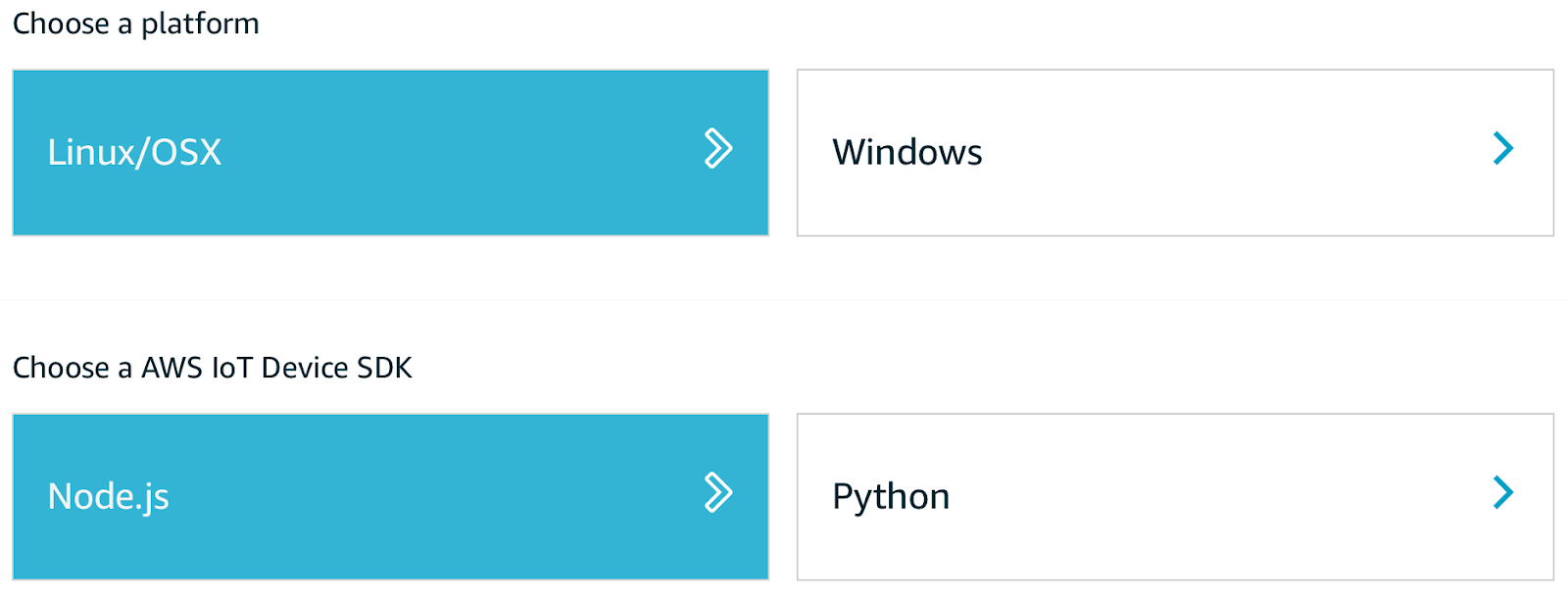
*Select OS and Language for downloading the connection kit*

Once downloaded, initialize a new Node.js project and install AWS-IoT-device-SDK. After that, it is possible to run the included start.sh script, making sure all the certificates, downloaded alongside the kit, are in the same directory. We can now create a local script to send data to a topic, passing the required modules and usingdevice.publish ("<topic>", payload):

const deviceModule = require('aws-iot-device-sdk').device;
const cmdLineProcess = require('aws-iot-device-sdk/examples/lib/cmdline');
…
device.publish('topic', JSON.stringify(payload));

The data sent is structured in JSON format with the following structure:

{	
   “timestamp”: “YYYY-MM-DD HH:MM:SS”,
   “room_id”: “XXXX”,
   “temperature”: 99
}

To create a Firehose delivery stream go to the Kinesis firehose service dashboard in the AWS web console, click “Create delivery stream”, select a name, and then “Direct PUT or other sources” like in figure:

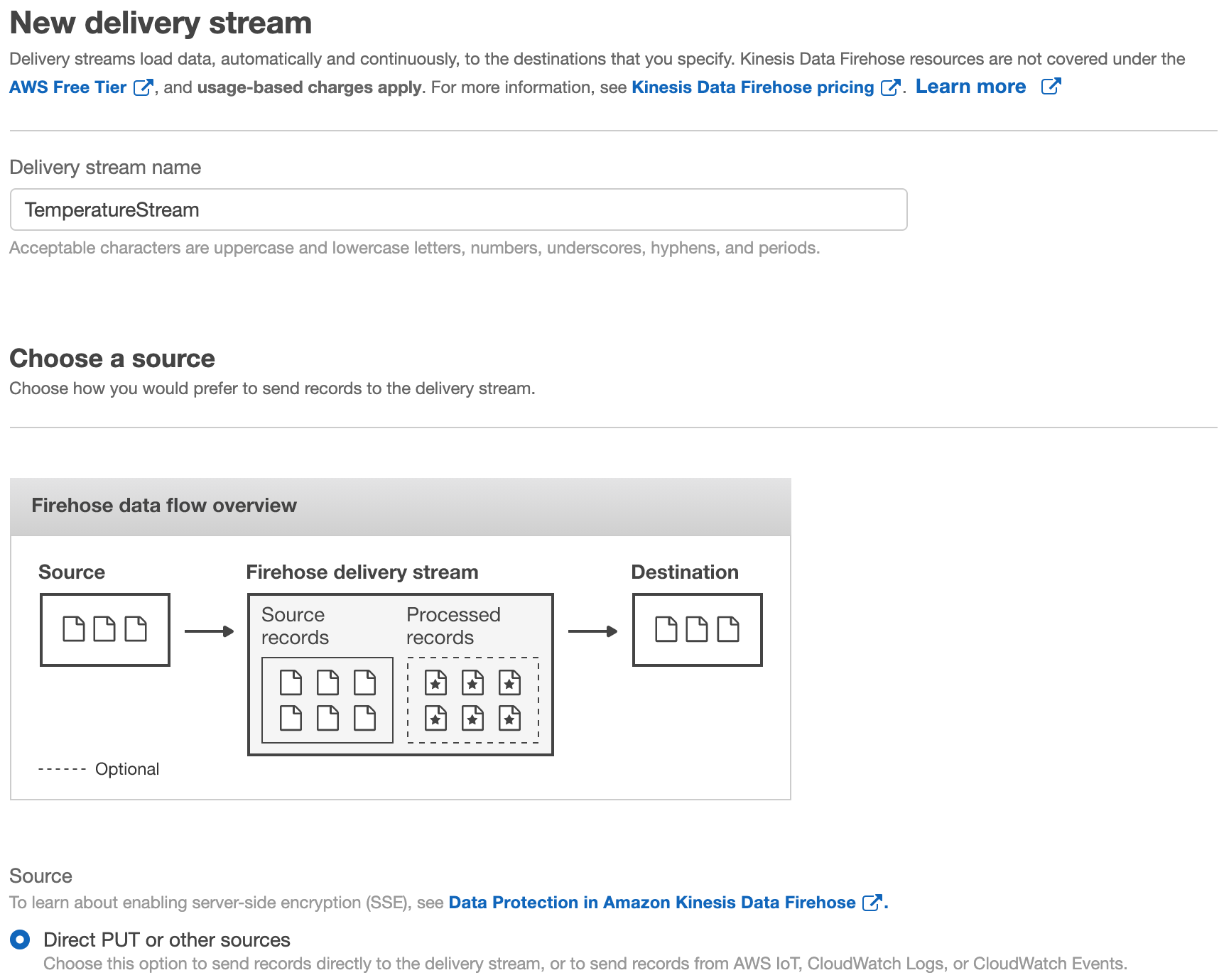
Leave “Data transformation” and “Record format conversion” as default. Choose an S3 destination as the target. Remember to also define an IoT Rule to send IoT messages to a Firehose delivery stream.

Glue crawlers and connectors

AWS Glue can be used to Extract and Transform data from a multitude of different data sources, thanks to the possibility of defining different types of connectors.

Database on EC2 instance

We want to be able to generate a Glue Data Catalog from a Microsoft SQL Server DB residing on an EC2 Instance in another VPC. To do so we need to create a JDBC connection, which can be done easily by going to the AWS Glue service page and by adding a new connection, found under the “Data Catalog - Databases” section of the sidebar menu.

Just add a name to the connection (which will be used by the related Crawler Job), the JDBC URL, following the right convention for ORACLE DBs, username and password, and the required VPC and subnet.

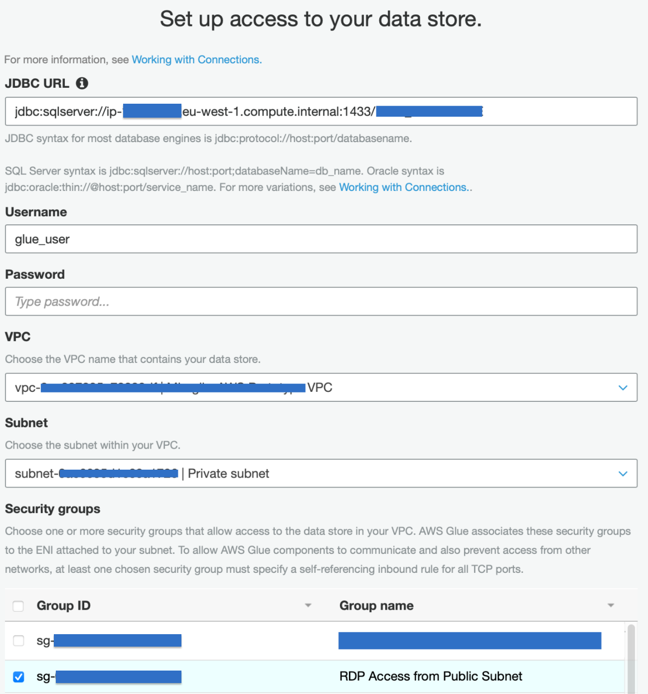
In order to establish a glue connection to the database, we need to create a new dedicated VPC that will be only used by Glue. The VPC is connected to the one containing the data-warehouse using VPC peering but other options are also possible, for example, we could have used AWS Transit Gateway. Once the peering is established remember to add routes to both the Glue and the DB subnets so that they can exchange traffic and to open the DB security group to allow incoming traffic on the relevant port from the Glue security group in the new VPC.

Data on S3

Data on S3 doesn’t need a connector and can be set up directly from the AWS Glue console. Create a new crawler, selecting “data stores” for the crawler source type; then check also “Crawl all folder”. After that is just a matter of setting the S3 bucket, the right IAM role and creating a new Glue Schema for this crawler. Also set “Run on demand”.

Glue Jobs

Glue jobs are the steps of the ETL pipeline. They allow extracting, transforming, and saving data back to a datalake. In our example, we would like to show two different approaches: jobs managed by AWS Glue Studio and using custom code. Both jobs will be later called by AWS Step Function.

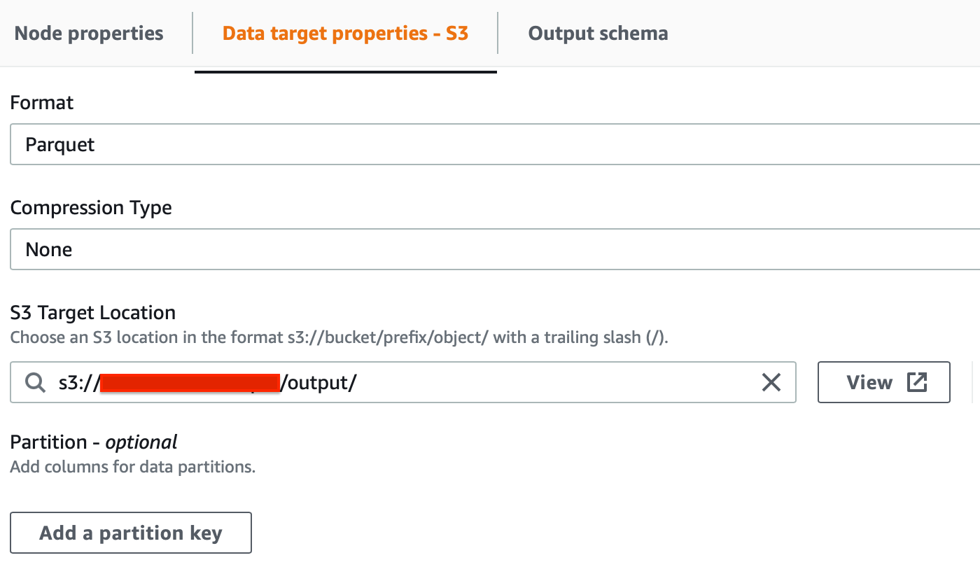
For historical data on S3, we can define Jobs from Glue Studio. For S3 select the following options in order:

On the Manage Jobs page, choose the source and target added to the graph option. Then, choose S3 for the Source and S3 for the Target.
Click on the S3 Data source, select the source bucket.
On the Node Properties tab, enter a name. Choose the Data source properties – S3 tab in the node details panel. Select your schema from the list of available databases in the Glue Data Catalog. Choose the correct table from the Catalog.
Verify the mapping is correct.
On the Node S3 Data target, select the output bucket, CSV as format (parquet is better, but we need CSV for Random Cut forest), no compression.

In order to extract data from our EC2 instance instead, we need a custom job. To create it we need to write a script ourselves, don’t worry, it’s fairly easy! Here are the key points you need to know to create a Spark Job with Glue: the ETL process is composed of 6 distinct areas in the script:

Import libraries

Basic set needed for a script:

import sys
from awsglue.transforms import *
from awsglue.utils import getResolvedOptions
from pyspark.context import SparkContext
from awsglue.context import GlueContext
from awsglue.job import Job
from awsglue.dynamicframe import DynamicFrame

Prepare connectors and other variables

To be used inside the script:

args = getResolvedOptions(sys.argv, ['JOB_NAME'])
sc = SparkContext()
glueContext = GlueContext(sc)
spark = glueContext.spark_session
job = Job(glueContext)
job.init(args['JOB_NAME'], args)

Get Dynamic Frames out of a Glue Catalog obtained by a Crawler

Use these dynamic frames to perform queries and transform data

rooms_temperatures_df = glueContext.create_dynamic_frame.from_catalog(database = "raw_temperatures", table_name = "temperatures", transformation_ctx = "temperature_transforms").toDF()
rooms_temperatures_df.createOrReplaceTempView("TEMPERATURES")

The last line enables modifying the dynamic frame.

Apply SQL operations

To extract distinct information

result = glueContext.sql("”)

In our case, we needed to generate 3 distinct results, one for each room using a simple WHERE room_id = <value>

Apply mapping

To generate a conversion schema

dynamicFrameResult = DynamicFrame.fromDF(result, glueContext, "Result")
applymapping = ApplyMapping.apply(frame = dynamicFrameResult, mappings = [("temp", "bigint", "temp","bigint"), ("room_id", "string", "room_id","string"), ("timestamp", "string", "timestamp","string")])

Save back to S3

To manipulate data later on

to_be_written = glueContext.write_dynamic_frame.from_options(frame = applymapping, connection_type = "s3", connection_options = {"path": "s3://", "partitionKeys": ["timestamp"]}, format = "csv", transformation_ctx = "to_be_written")
job.commit()

Step Function

Step function represents the core, the logic of our sample solution. Its main purpose is to manage all the ETL jobs, keep them synchronized, and manage errors. One advantage is that we can use Step Function to regulate the data being injected into the central S3 bucket which is where we save all cleaned data.

To start, this is the step function schema we used for this example:

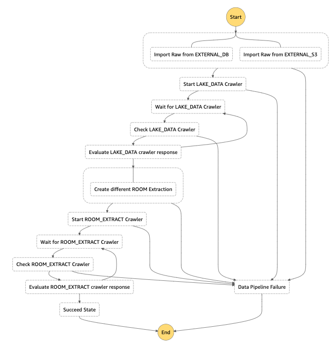
In our example there are a couple of things we would like to share about Step Function; firstly we have 2 main crawler loops: the first one, has branches and runs 2 crawlers (one for S3 standard, and one for the EC2 database which is the custom one); the second one takes all the data retrieved from both historical data sources and live one (from Kinesis Firehose), and extract per-room datasets in order to use them with Amazon SageMaker.

As Crawlers are asynchronous we can’t wait for them so we needed to create 2 waiting loops for both of the execution steps

AWS Lambda is used to call AWS Glue APIs in order to start the jobs we have configured before.

To give a hint here are some interesting parts described in the JSON file representing the state machine.

"Type": "Parallel",
  "Branches": [
        {
          "StartAt": "Import Raw from EXTERNAL_DB",
          "States": {
            "Import Raw from EXTERNAL_DB": {
              "Type": "Task",
              "Resource": "arn:aws:states:::glue:startJobRun.sync",

In AWS Step Function, we can launch tasks in parallel (for us, the two historical data glue jobs) using “Type: Parallel” and “Branches”. Also after the key “Branches”, it is possible to retrieve the parallel result.

"ResultPath": "$.ParallelExecutionOutput",
"Next": "Start LAKE_DATA Crawler"

We can run a synchronous Glue job defined in the console by passing the job’s name, and you can also enable the generation of a glue catalog during the process.

"Parameters": {
                "JobName": "EXTERNAL_DB_IMPORT_TO_RAW",
                "Arguments": {
                  "--enable-glue-datacatalog": "true",

It is possible to catch exceptions directly in Step Function by moving to an error state using “Catch”:

"Catch": [
        {
          "ErrorEquals": [
            "States.TaskFailed"
          ],
          "Next": "Data Pipeline Failure"
        }
],

Because we don’t have a standard way to wait for the jobs to finish, we use the parallel jobs output and a StepFunctions wait cycle to check if the operation is done; for that, we use the “Wait” key:

"Wait for LAKE_DATA Crawler": {
      "Type": "Wait",
      "Seconds": 5,
      "Next": "Check LAKE_DATA Crawler"
},

The rest of the flow is pretty much a repetition of these components.

The interesting fact is that we can apply some starting conditions to alter the execution of the flow, like avoiding some jobs if not needed at the moment or even run another state machine from a precise step to take our example and modularize the most complicated parts.

Athena and Quicksight

Athena can generate tables that can be queried using standard SQL language, not only: results of Athena queries can be imported into Amazon Quicksight to rapidly generate charts and reports, based on your data.

In our workflow, it is possible to run Athena queries on the target S3 bucket which contains both global temperature data and sensor’s specific ones. Let’s review quickly how to do that:

If you have already created a Glue Crawler, you’ll have a Datasource and a table.
Select the database and table in Athena’s dashboard in the left sidebar (we used temperatures_db and temperatures from our crawlers).
Create a simple query that can later be used by QuickSight to show a chart, for example, a simple “SELECT * FROM temperatures”.

By doing these 3 steps Athena will show the result of the query as shown below:

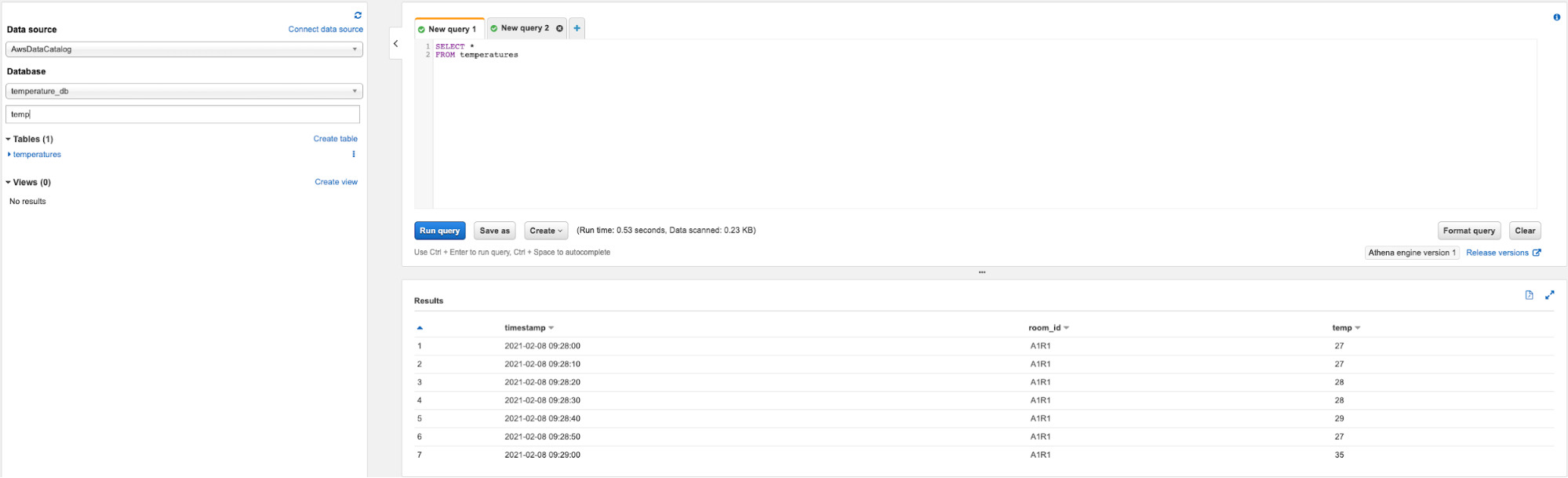
A couple of tips when working with Athena:

Avoid using “-” in the database’s name, use “_” instead.
When possible avoid crawlers to scan folders containing files with different schemas, only scan for files with the same schema (if you need to do partitions for example).

Quicksight can read Athena’s query and present charts and diagrams from them. It’s very straightforward: just go to the Quicksight service’s page and follow one of the many tutorials about it, keeping in mind a few important things:

Quicksight is not directly included in your account’s resources, you must enable a paid subscription (there is a 60 days trial though).
To access Athena, Quicksight needs its role to be modified with full access to Athena.
An SSL valid certificate must be issued, for example using Amazon ACM.

If you don’t want or can’t use Quicksight, you can always call Athena’s API directly and build your own dashboard from data.

Sagemaker: Random Cut Forest anomaly detection

The machine learning algorithm we will explore in this article is called Random Cut Forest. The algorithm takes a bunch of random data points (Random), cuts them to the same number of points, and creates trees (Cut). Finally, it checks all the trees together (Forest) to verify if a particular data point is to be considered an anomaly.

Generally speaking, a tree is an ordered way of storing numerical data, and to create it, we randomly subdivide the data points until it is possible to isolate the point we’re testing to determine whether it’s an anomaly. A new level of the tree is created whenever we subdivide the points.

Sagemaker offers a built-in implementation of Random Cut forest which accepts data points in CSV format. We can retrieve them easily with:

data_location = f”s3://{bucket}/{key}”
df=pd.read_csv(data_location,delimiter=’,’)

Data contains a timestamp, the temperature value in C°, and aroom_id, which identifies a particular room where the sensor was installed. We have already used our Step Function to divide data coming from different rooms so we can directly pass the CSV to the Estimator.

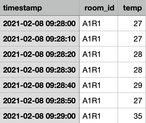
Sample data extract We referred to this article to verify how data must be passed to the Estimator. According to the official documentation, we need to pass 3 main hyperparameters:

num_samples_per_tree - the number of randomly sampled data points sent to each tree. 1/num_samples_per_tree should approximate the estimated ratio of anomalies/points in the dataset.
num_trees - the number of trees to create in the forest. Each tree learns a separate model from different samples of data.
feature_dim - the dimension of each data point.

The Estimator is defined in this way:

import sagemaker
from sagemaker import RandomCutForest
 
execution_role = sagemaker.get_execution_role()
sagemaker_session = sagemaker.Session()
bucket = “”
prefix = “”
 
rcf = RandomCutForest(
    role=execution_role,
    instance_count=1,
    instance_type="ml.m4.xlarge",
    data_location=f"s3://{bucket}/{prefix}",
    output_path=f"s3://{bucket}/{prefix}/output",
    num_samples_per_tree=512,
    num_trees=50,
)
rcf.fit(rcf.record_set(df.value.to_numpy().reshape(-1, 1)))

Some considerations to take into account are that we generate the execution_role and thesagemaker_session using the built-in methods. For our training, we use an ml.m4xlarge instance, while for inference we used an ml.c5.xlarge as suggested by the docs. Don’t’ waste credits on GPU instances as the RCF algorithm doesn’t take GPU into account.

For deploying we can use the standard approach:

rcf.deploy(initial_instance_count=1, instance_type="ml.m4.xlarge")

And that’s it! We have reached the end of this workflow. Let’s see some references and sum up all we have seen until now.

References

Takeaways

In this article, we have seen many services from AWS perfectly suited for data analytics when dealing with near real-time scenarios. We have discussed about AWS Step function and how it can be used to orchestrate nonlinear workflows, giving developers the ability to have multiple choices in manipulating and extracting data for different kinds of analysis.

AWS Glue proved to be flexible enough to take care of data sources residing in different places: EC2 instances, S3, and in different accounts. It was a perfect choice also due to the simplicity of setting up Spark jobs. We have seen in particular how to connect to a data source using a JDBC connection.

Athena demonstrated to be the perfect tool to extract ETL results for Business Intelligence fruition, and Quicksight the obvious choice to show the results, as it’s natively compatible with Athena queries.

As in many other scenarios we have faced, Kinesis Data Firehose was also used to transfer near real-time data to S3 from a non-AWS source.

We have also seen how Amazon S3 is always a must-have when dealing with big data workflows, machine learning problems, and data lake creation. Its durability standards, as well as its being compatible with any other AWS service, makes it the perfect choice both for long term storage and in-between steps buffer.

To conclude we gave some hints on how to manipulate data in SageMaker to carry out inference for anomaly detection.

This concludes our journey for today, as always feel free to comment and reach us to discuss any question, doubt, or idea that comes to your mind. We’ll be glad to respond as soon as possible!

Stay tuned: another story's coming in 14 days on #Proud2beCloud! :) See you there!

Matteo Moroni

DevOps and Solution Architect at beSharp, I deal with developing Saas, Data Analysis, and HPC solutions, and with the design of unconventional architectures with different complexity. Passionate about computer science and physics, I have always worked in the first and I have a PhD in the second. Talking about anything technical and nerdy makes me happy!

Alessandro Gaggia

Head of software development at beSharp and Full-Stack Developer, I keep all our codebases up-to-date. I write code in almost any language, but Typescript is my favorite. I live for IT, Game design, Cinema, Comics, and... good food. Drawing is my passion!