AWS Data Transfer Costs: from “a nutshell” to the calculator through 3 real-world scenarios

In the previous article: "AWS data transfer costs in a nutshell" we explored AWS network costs in detail: inbound and outbound data transfer, traffic between Regions and Availability Zones, VPC peering, NAT Gateways, and VPC Endpoints.

The theory is clear, but how does it translate into practice?

It's time to move from abstraction to reality. In this article, we'll analyze three real-world scenarios of increasing complexity, demonstrating how a proper network cost analysis can lead to significant savings and more informed architectural decisions.

Get your Jupyter Notebooks ready: it's time to do the math.

Case 1: MongoDB Atlas - Public Endpoint vs VPC Peering

The context

An application hosted on AWS uses MongoDB Atlas as its database. Currently, access is via public endpoints, but we're asked to evaluate whether it's worth investing time in setting up a VPC peering to the VPC provided by MongoDB.

The substantial difference between the two solutions lies in the network path:

• Public Endpoint: traffic leaves the VPC through a NAT Gateway, reaches MongoDB Atlas over the internet, and incurs related charges
• VPC Peering: traffic remains private, travels over the AWS peering connection, and avoids NAT Gateway costs

Cost analysis

Let's consider a MongoDB M10 instance ($57/month) and analyze the network costs for both solutions.

Solution A - Public Endpoint

Costs include:

• M10 Cluster: $57/month
• NAT Gateway: $0.048/h
• NAT Gateway data processing: $0.048/GB
• Data transfer OUT: $0.09/GB

The total cost formula is:

Cost_SaaS-M10 = Cluster_M10 + NAT_hourly × 730 + V × (NAT_processing + Internet_out)

where V represents the monthly traffic volume (V will have the same meaning for the following formulas).

Solution B - VPC Peering

MongoDB Atlas does not charge for VPC peering. Charges are limited to AWS traffic:

• M10 Cluster: $57/month
• VPC Peering same-AZ: free
• Cross-AZ VPC Peering: $0.01/GB (both directions)

A complication arises here: Availability Zones are not aligned across different AWS accounts. The identifier eu-west-1a in our account does not necessarily correspond to eu-west-1a in the MongoDB account. Without being able to guarantee same-AZ placement, we must assume cross-AZ traffic.

The formula becomes:

Cost_Peering-M10 = Cluster_M10 + V × (CrossAZ_in + CrossAZ_out)

Use: Cross-AZ traffic costs $0.01/GB in both directions (in and out of AZ), for a total of $0.02/GB on peering.

Comparison and Results

Let's calculate the cost difference:

ΔCost_M10(V) = Cost_SaaS-M10 − Cost_Peering-M10
ΔCost_M10(V) = [Cluster_M10 + NAT_hourly × 730 + V × (NAT_processing + Internet_out)] − [Cluster_M10 + V × (CrossAZ_in + CrossAZ_out)]
ΔCost_M10(V) = NAT_hourly × 730 + V × [(NAT_processing + Internet_out) − (CrossAZ_in + CrossAZ_out)]
ΔCost_M10(V) = $35.04 + V × 0.118

The result is always positive: VPC peering generates savings in every traffic scenario.

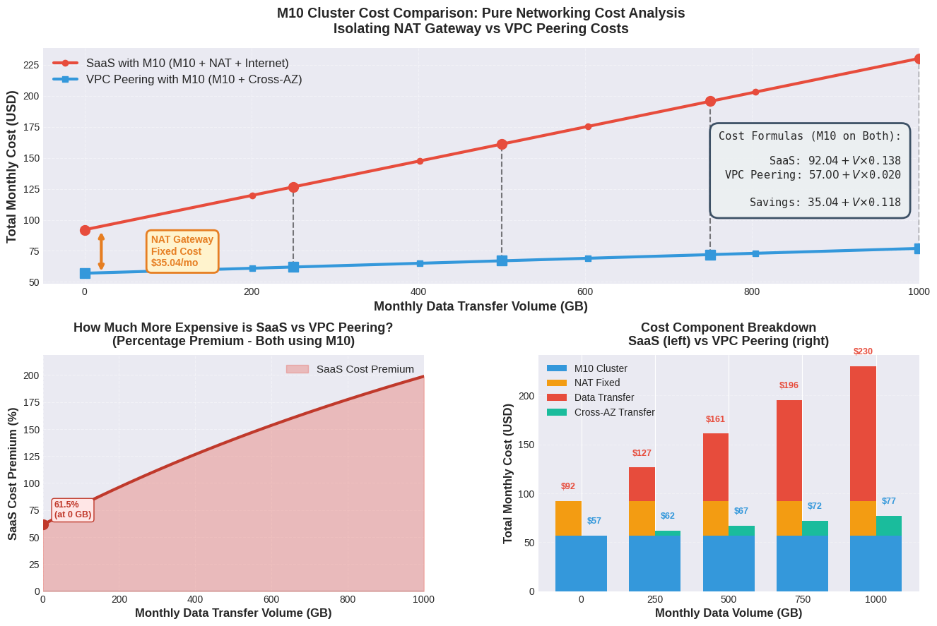
The graph highlights two fundamental aspects:

1. Fixed basic savings: the cost of the NAT Gateway alone ($32.85/month) represents an immediate saving, regardless of traffic volume
2. Marginal savings: each GB transferred costs $0.118 less with peering

Even with very high traffic volumes (over 10TB/month), the cost of cross-AZ data transfer on peering does not even reach the cost of the NAT Gateway alone of the public solution.

Conclusions

VPC peering to MongoDB Atlas is cost-effective for any traffic scenario. In addition to the economic benefits, there are:

• Safety: traffic remains in the AWS private network
• Performance: lower latency and more stable throughput than the public network
• Simplicity: Deleting a NAT Gateway and Managing It

It is worth noting that, even assuming cross-AZ traffic (worst-case scenario), there is a statistical probability of obtaining a same-AZ matching, which would make the savings even greater thanks to the absence of peering costs.

Case 2: AWS S3 Backup - Private vs Public Connectivity

The context

A client commissioned us to design an architecture to back up on-premise servers to S3. The requirements were:

1. "Keep traffic private by switching to Direct Connect"
2. "Contain costs"

The customer already has a Direct Connect connection to AWS with a Transit Gateway configured.

Questioning the requirements

As always in architecture, it is essential to validate requirements before accepting them uncritically.

We understand the reasoning: having already invested in a Direct Connect, it seems logical to use it for every use case. However, for traffic to S3, AWS provides optimized public connectivity and, more importantly, Data transfer IN to AWS is free.

The question becomes: how much does this traffic “privacy” really cost?

Cost analysis

In this case, our variable will be the volume in GB to be backed up to S3 Standard on a monthly basis.

Solution A - Private Traffic via Direct Connect

The traffic route is:

On-premise → Direct Connect → Transit Gateway → VPC → VPC Endpoint (S3) → S3

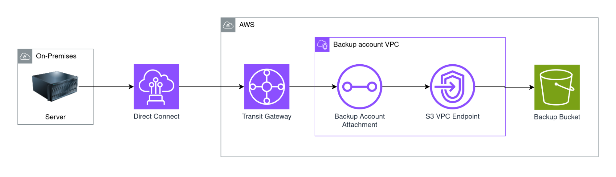
Costs include:

• Direct Connect: $0.30/h (already existing)
• Transit Gateway attachment: $0.05/h
• Transit Gateway data processing: $0.02/GB
• VPC Endpoint for S3: Free
• S3 storage: $0.023/GB-month
• S3 API calls: negligible cost for comparison purposes as it is identical in both solutions

Therefore the total cost of option A is:

Cost_Private = DCPortHours + TGAttachment_hourly × 730 + (V × TG_processing) + S3Storage + S3API
Cost_Private = $219 + $36.50 + (V × $0.02) + S3Storage + API Costs
Cost_Private = $255.50 + (V × $0.02) + S3Storage + API Costs

In fact, if Direct Connect is already present, it is possible to exclude it from the total cost:

Cost_Private = $36.50 + (V × $0.02) + S3Storage + API Costs

Solution B - Public Traffic

The path is simply:

On-premise → Internet → S3

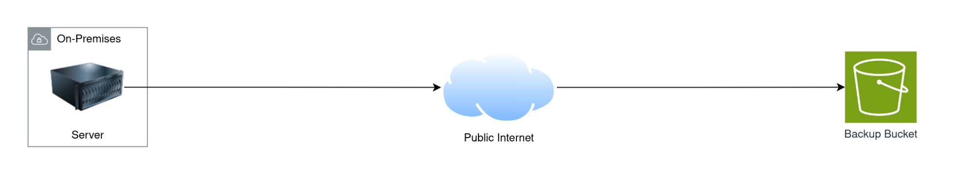
The costs are:

• Data IN to AWS: Free
• S3 storage: $0.023/GB-month
• S3 API calls: negligible cost for comparison purposes as it is identical in both solutions

Cost_Public = S3Storage + S3API

Comparison and Results

At this point it is very simple to make the difference between the two costs:

ΔCost(V) = Cost_Private − Cost_Public
ΔCost(V) = $36.50 + (V × $0.02)

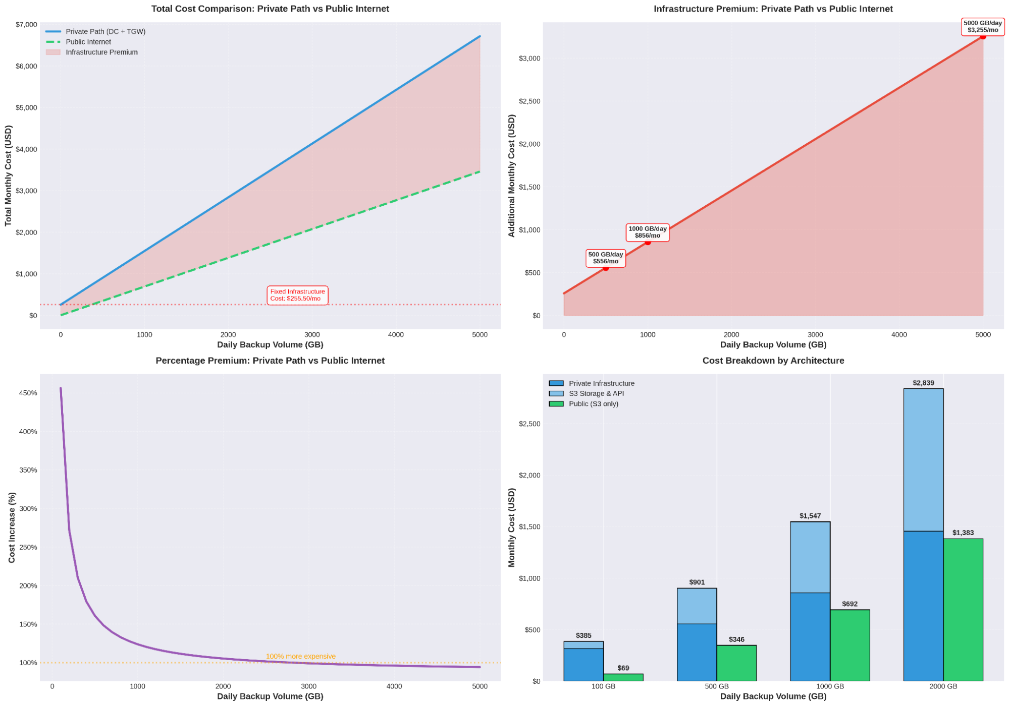
The graphic analysis reveals an unequivocal picture:

1. For small volumes (hundreds of GB): the private solution costs several times more than the public solution. The fixed cost of the Transit Gateway attachment ($35/month) dominates the total cost.
2. For high volumes (tens of TB): the cost of the private solution stabilizes at approximately double the public solution. The variable component ($0.02/GB of Transit Gateway processing) represents a constant overhead.

There is no break-even point: the public solution is always more cost-effective, regardless of data volume.

Additional considerations

Alternatives not analyzed in detail:

For completeness, we mention a third option: using an AWS Direct Connect Public VIF instead of the Private VIF with Transit Gateway. This solution keeps traffic on the dedicated Direct Connect connection (avoiding transit over the public internet) but eliminates the need for the Transit Gateway, significantly reducing costs. A detailed analysis of this option is beyond the scope of this article, but it represents an interesting alternative for specific contexts.

When the private solution makes sense:

Economic analysis is not the only factor in the decision. A private solution can be justified in the presence of:

• Compliance requirements that impose private traffic
• Stringent corporate security policies
• Limitations of available on-premise internet bandwidth
• Need for guaranteed QoS

Conclusions

From a purely economic standpoint, the public solution is superior in every scenario. The savings range from a factor of 5-10x for small volumes to a factor of 2x for large volumes.

Case 3: NAT Gateways - Centralized or Distributed?

The context

An AWS organization with dozens of accounts finds itself managing a large number of distributed NAT Gateways. Each account has a VPC with three NAT Gateways (one per Availability Zone), generating significant monthly costs even when there is no traffic.

The question arises spontaneously: does it make sense to maintain a NAT Gateway in each account, or is it better to centralize internet egress in a dedicated account, reachable from other accounts via a Transit Gateway?

Important premise

This architectural decision has implications that go beyond the purely economic aspect:

• Traffic inspection: centralizing allows you to implement centralized security controls
• IP addressing: allows you to use company-owned public IPs for all outgoing traffic
• Governance: facilitates audit and compliance by centralizing the egress point
• Blast radius: a centralized NAT Gateway issue impacts all accounts.

In this article, we will focus exclusively on economic analysis, but it is essential to consider these aspects in a real evaluation.

Cost analysis

Let's consider an organization with N AWS ​​accounts, each with a VPC and three NAT Gateways (one per AZ).

Solution A - Distributed NAT Gateways

Each account has:

• 3 NAT Gateway: 3 × $0.048/h
• NAT Gateway data processing: $0.048/GB
• Data transfer OUT: $0.09/GB

Cost_Distributed = N × (NAT_{per_AZ} × AZCount × NAT_hourly × 730 + V_{per_account} × NAT_processing) + V × Internet_out

Substituting some variables we arrive at:

Cost_Distributed = N × (3 × $0.048 × 730 + V_{per_account} × $0.048) + V × Internet_out
Cost_Distributed = N × ($105.12 + V_{per_account} × $0.048) + InternetEgressCost

We leave the cost of outgoing traffic expressed as a variable, as it will also be present in the second case, therefore it is not necessary to calculate it for comparison purposes.

Solution B - Centralized NAT Gateways

Architecture:

VPC spoke → Transit Gateway → VPC egress → NAT Gateway → Internet

Costs involved:

• Transit Gateway attachments: $0.05/h × (N spoke + 1 egress) account
• Centralized NAT Gateways: 3 × $0.048/h
• Transit Gateway data processing: $0.02/GB
• NAT Gateway data processing: $0.048/GB
• Data transfer OUT: $0.09/GB

Cost_Centralized = (N + 1) × TGAttachment_hourly × 730 + NAT_count × NAT_hourly × 730 + V × (TG_processing + NAT_processing + Internet_out)

Substituting some variables we arrive at:

Cost_Centralized = (N + 1) × $0.05 × 730 + 3 × $0.048 × 730 + V × ($0.02 + $0.048) + InternetEgressCost
Cost_Centralized = (N + 1) × $36.50 + $105.12 + V × $0.068 + InternetEgressCost
Cost_Centralized = ($36.50 + $105.12) + N × $36.50 + V × $0.068 + InternetEgressCost
Cost_Centralized = $141.62 + N × $36.50 + V × $0.068 + InternetEgressCost

Two-dimensional Analysis

We're dealing with a function with two variables: traffic and number of accounts. We need to analyze both.

Chart 1 - Fixed Traffic, Variable AccountTwo-dimensional Analysis

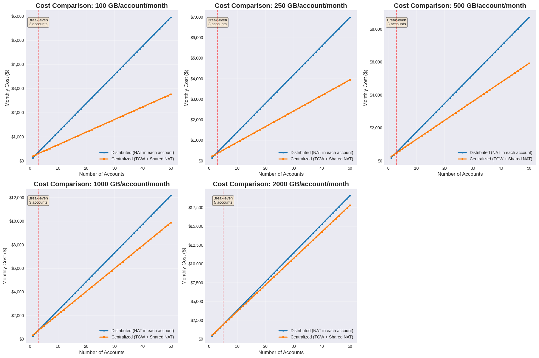
By setting the traffic volume at different levels (1TB, 5TB, 10TB, 50TB, 100TB), we observe that:

1. For low traffic volumes: break-even is achieved with very few accounts. From that point on, centralization generates increasing savings.
2. For high volumes: the break-even point is slightly higher due to the additional $0.02/GB cost of Transit Gateway processing.
3. Maximum savings: this is achieved with many accounts and little traffic per account.

Graph 2 - Three-dimensional Visualization

If we want to avoid fixing the traffic variable, a two-dimensional graph is no longer sufficient; we must therefore move from a straight line to a plane. The three-dimensional graph offers a complete view of the cost trend as both variables vary simultaneously.

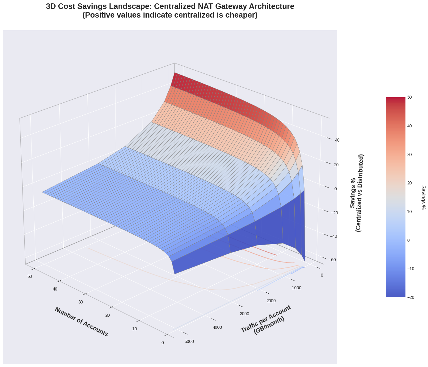
The three-dimensional graph shows the same trend as above. The greatest savings are achieved with a high number of accounts and low traffic.
This graph highlights another interesting piece of information: although very high amounts of traffic can make centralizing NAT Gateways not very economically advantageous, for accounts with more than ten accounts it is almost impossible to find yourself in this situation.

Chart 3 - Simplification for Readability

The three-dimensional graph, although complete, can be difficult to read. To simplify the visualization, we have created a two-dimensional graph that shows the cost difference (green zone = savings, red zone = additional cost) as a function of account and traffic.

Conclusions

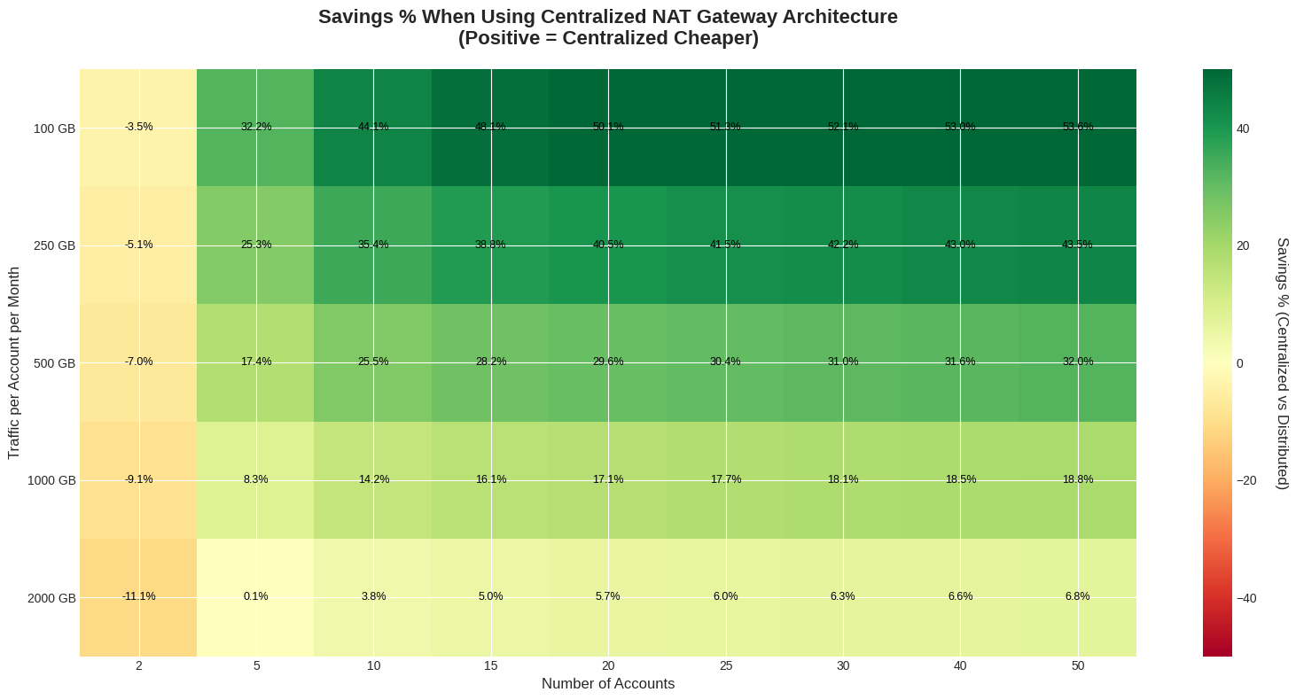
The economic analysis clearly indicates that centralizing NAT Gateways is cost-effective in most real-world scenarios, in particular:

Centralization is convenient when:

• You have 5+ accounts in your organization
• Traffic per account is moderate (<5TB/account/month)
• You want to achieve increasing savings with scale

Distribution may be preferable in the rare situations where:

• You have very few accounts (<3-4)
• Traffic per account is extremely high (>50TB/account/month)
• There are very stringent isolation or blast radius requirements

General conclusions

Through these three real-world cases, we've shown that careful analysis of AWS network costs can lead to significant savings and more informed architectural decisions. The key lesson is clear: question initial requirements and validate them with concrete data, even when they appear to stem from logical choices or investments already made. Fixed costs like NAT Gateway and Transit Gateway have a huge impact on workloads with limited traffic, while the scale of the organization can completely overturn the economics. The time invested in initial optimization typically pays for itself within a few months of operation.

About Proud2beCloud

Proud2beCloud is a blog by beSharp, an Italian APN Premier Consulting Partner expert in designing, implementing, and managing complex Cloud infrastructures and advanced services on AWS. Before being writers, we are Cloud Experts working daily with AWS services since 2007. We are hungry readers, innovative builders, and gem-seekers. On Proud2beCloud, we regularly share our best AWS pro tips, configuration insights, in-depth news, tips&tricks, how-tos, and many other resources. Take part in the discussion!